背景
偶然从墙头掉下去看见泰瑞陶的博客有一篇Tsunami模拟的文章,原来,浅水波公式是海啸数学模拟的基础.
然后就开始好奇,如果物理原理都是确定的,那么什么样的地震能够产生何种海啸? 现在的数学模型到底能模拟出什么样子? 看上去模型刚好是一个transient partial differential equations system, 可以用methods of lines 求解的类型, 就寻思, Mathematica最擅长这个了,有没有这方面的例子?
在热心网友JM的帮助下,还真找到了.
内容
在Wolfram有一帮这样的科学家或工程师, 负责内核技术(, Kernel Technology) 开发的 Rob Knapp发表过如下博客文章介绍NDSolve的使用(2007年海啸Sumatra有关)
作者主要工作是Mathematica求解微分方程数值解; Wolfram致力于各种微分方程(组)的自动求解, 即用户可以直接输入他们的微分方程(方程组), Mathematica对此进行分析判断并采用最佳的方法来求解. (喜欢这种思路)
http://blog.wolfram.com/2007/09/13/not-another-tsunami/
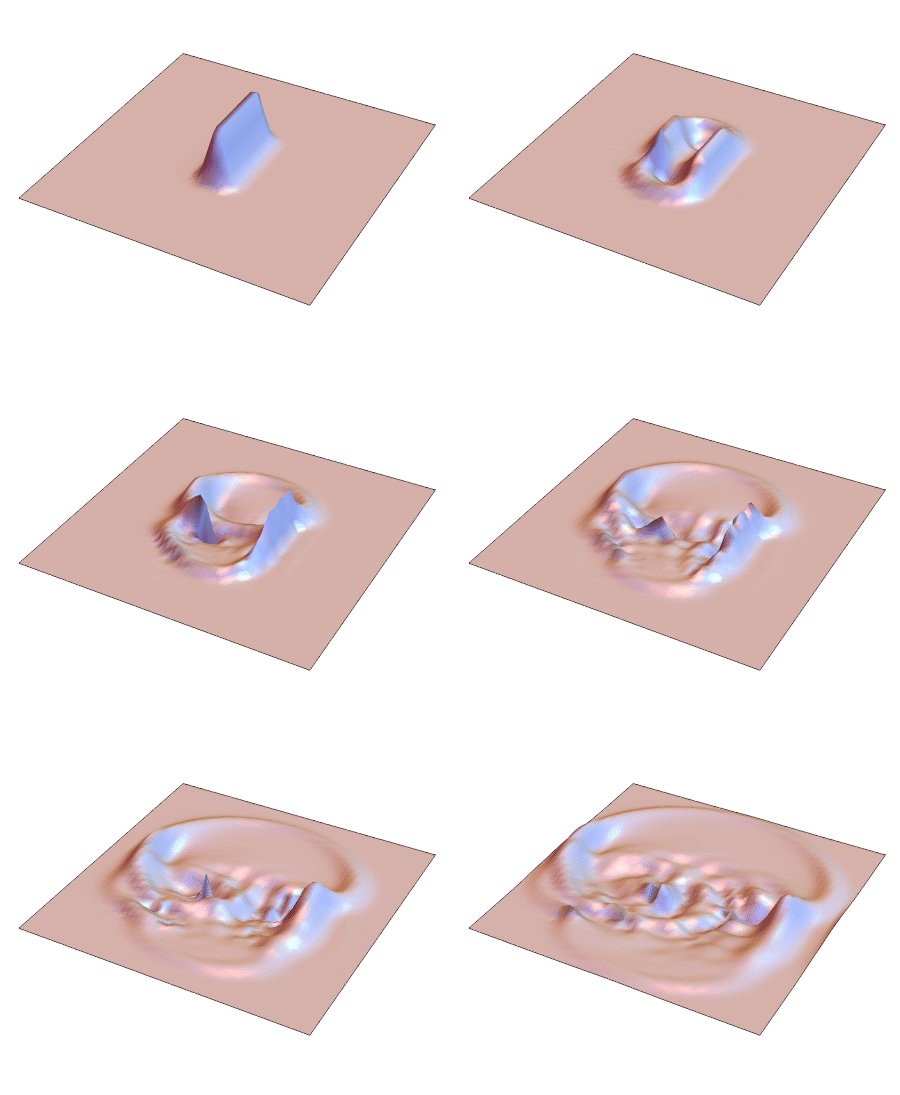
下面是模拟出的波动的效果,看上去酷似泥水塘里坠入大石块之后翻起的波浪,放大了之后能够成为海啸?
Today’s earthquakes near Sumatra fortunately didn’t lead to a major tsunami. But figuring out when tsunamis will develop is a difficult matter–and an interesting exercise in applied mathematics.
The main phenomenon is the propagation of so-called shallow water waves–water waves whose wavelength is large compared to the depth of the ocean. Those waves satisfy a partial differential equation (PDE) that was figured out in the 1800s. The equation is a nasty nonlinear one–that can’t be solved exactly.
I’ve been working on the numerical differential equation capabilities of Mathematica for more than a decade. Our goal is to automate the solutions of all types of equations–so users just have to enter their equation, and Mathematica then does all the analysis to select and apply the best algorithm.
The shallow-water equations are a good test–that I’m happy to say Mathematica passes with flying colors. One essentially just has to type the equations in, and get the solution, which is then easy to visualize–especially using the new visualization capabilities of Mathematica 6. (Click the image below to see the Mathematica animation.)
Click for Tsunami Animation Exported from Mathematica
Let me explain a little about what’s involved in getting this.
Here’s an image of a Mathematica notebook that produces the main picture (you can download the notebook here):
Mathematica Notebook of Tsunami Visualization
The first thing is just the equations, given in Mathematica StandardForm (one could use TraditionalForm so it looks exactly like a traditional textbook, but it’s slightly harder to understand that way). Then we just use NDSolve to solve the equations. Then we use Plot3D to create a 3D visualization–complete with specular surfaces and everything. And finally, we use Animate to create an animation. (We can immediately export for the web using Export.)
What’s going on inside NDSolve? That one function is doing some pretty complicated things–it’s almost a microcosm of a century or two of applied mathematics.
NDSolve is doing a lot of things that can really only be done in Mathematica–by combining Mathematica‘s strength not only in numerical computation, but also in symbolic computation and discrete mathematics.
That you can just type an equation into NDSolve relies on Mathematica‘s general symbolic architecture. Once NDSolve gets an equation, it immediately determines the structure. In this case, it finds out that it’s been given a (2+1)-dimensional initial-value PDE.
For that type of equation, it forms a discrete grid in space (with the grid structure determined automatically to meet a certain accuracy criterion), then generates a large system of first-order ODEs on that grid, automatically incorporating all the necessary boundary conditions.
NDSolve has about 20 different families of methods for solving ODEs. In this case, it actually switches automatically between explicit and implicit methods depending on local stiffness. (The implicit methods get to use some of our very fast sparse matrix solving capabilities.)
In the end, NDSolve packages its solution as an InterpolatingFunction–a very convenient Mathematica construct that directly represents an approximate function, that in this case we chose to plot using Plot3D.
(Even though NDSolve can figure out what to do automatically, you can always give it hints, or even tell it exactly what method to use. In this case, you can improve the quality of the solution by choosing to use a pseudospectral method with a specified number of grid points.)
As one of the people responsible for NDSolve, I know how complicated all the things it does inside are. But when you use NDSolve, all you have to do is type your equation in, and let Mathematica do the rest. We’ve done the work (and it’s been a lot of work, I might add) to have everything run efficiently and automatically from there.
It might take a while to work out the physics of the shallow water wave approximation to a tsunami. But I think I can say that Mathematica‘s part of solving the equations could be accomplished before a tsunami has propagated very far.


 5081
5081

 被折叠的 条评论
为什么被折叠?


