MATLAB 实现 Cox 生存分析与风险分组：完整代码与解析

原创于 2025-03-14 15:29:38 发布 · 737 阅读

6 ·

CC 4.0 BY-SA版权

文章标签：

#matlab #开发语言

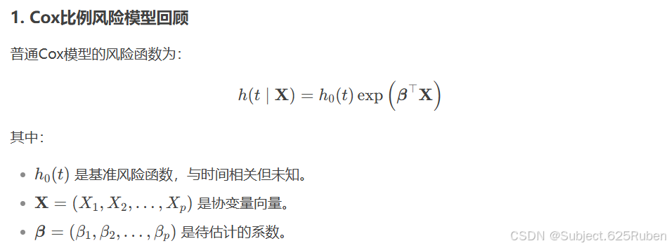
在生存分析中，Cox 比例风险回归模型（Cox Proportional Hazards Model）是一种常用的统计方法，可用于评估多个变量对生存时间的影响。

本篇博客将介绍如何使用 MATLAB 构造模拟生存数据，并应用 Cox 模型进行分析，包括：

生成模拟数据（基于肺癌数据集格式）
处理缺失值
拟合 Cox 回归模型
计算风险评分并进行分组
使用 Kaplan-Meier 估计绘制生存曲线
进行 Log-Rank 检验

1. 生成模拟生存数据

首先，我们创建一个模拟数据集，包括生存时间（time）、生存状态（status）、年龄（age）以及 ph.ecog 评分（反映患者体能状况）。

数据示例（删除缺失值后的 cleanData）：

time	status	age	ph_ecog
315.2	1	65	2
278.4	0	52	1
322.7	1	74	3

2. Cox 回归模型

Cox 模型用于评估 age 和 ph.ecog 对生存时间的影响。在 MATLAB 中，使用 coxphfit 函数进行拟合。

3. 计算风险评分并分组

Cox 模型的线性预测值（风险评分）计算。

示例数据：

time	status	age	ph_ecog	risk_score	risk_group
315.2	1	65	2	0.62	middle
278.4	0	52	1	0.21	low
322.7	1	74	3	1.32	high

4. Kaplan-Meier 生存曲线

我们使用 kmplot 自定义函数绘制 Kaplan-Meier 生存曲线，观察不同风险组的生存情况。

figure;
hold on;
groups = categories(cleanData.risk_group);
colors = [0.9 0.5 0; 0.4 0.6 0.2; 0 0.4 0.8]; % 橙、绿、蓝

for i = 1:length(groups)
    idx = (cleanData.risk_group == groups{i});
    kmplot(time(idx), status(idx),...
        'Color', colors(i,:), 'LineWidth', 2, 'DisplayName', groups{i});
end

title('生存分析：低、中、高风险组');
xlabel('时间'); ylabel('生存概率');
legend('Location', 'best'); grid on;
hold off;

kmplot 函数

function [S, T] = kmplot(time, status, varargin)
% 计算生存函数
[S, T] = ecdf(time, 'censoring', ~status, 'function', 'survivor');

% 解析绘图参数
p = inputParser;
addParameter(p, 'Color', [0 0.447 0.741], @isnumeric);
addParameter(p, 'LineWidth', 1.5, @isnumeric);
addParameter(p, 'DisplayName', 'Group', @ischar);
parse(p, varargin{:});

% 绘制阶梯图
stairs(T, S, 'Color', p.Results.Color,...
    'LineWidth', p.Results.LineWidth,...
    'DisplayName', p.Results.DisplayName);
end

5. Log-Rank 检验

为了检验不同风险组的生存率是否存在显著差异，我们使用 Log-Rank 检验。

6. 结果解读

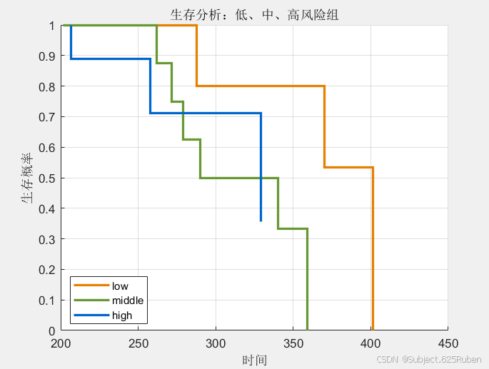
Cox 模型分析：发现 age 和 ph.ecog 影响生存率，且 ph.ecog 更显著。
生存曲线：风险评分高的患者生存率较低。
Log-Rank 检验：若 p 值 < 0.05，说明不同风险组之间生存差异显著。

完整代码：

% 生成示例数据（30条记录，格式与lung数据集一致）
rng(1); % 固定随机种子保证可重复性

% 明确创建列向量 (关键步骤)
time_col = abs(randn(30,1)*50 + 300);   % 确保时间为正数
status_col = randi([0 1],30,1);        % 状态（0=删失，1=事件）
age_col = randi([40,80],30,1);         % 年龄（40-80岁）
ph_ecog_col = randi([0,3],30,1);       % ph.ecog评分（0-3）

% 水平拼接为矩阵（30行×4列）
dataMatrix = [time_col, status_col, age_col, ph_ecog_col];

% 转换为表格并指定列名
sampleData = array2table(dataMatrix, 'VariableNames', {'time','status','age','ph_ecog'});

% 添加缺失值（模拟真实数据场景）
sampleData.ph_ecog(randi(30,2,1)) = NaN;
sampleData.age(randi(30,1,1)) = NaN;

% 删除缺失值
cleanData = rmmissing(sampleData);

% 提取协变量矩阵和时间-状态数据
X = [cleanData.age, cleanData.ph_ecog];
time = cleanData.time;
status = cleanData.status;

% ========== 关键修复部分 ==========
% 正确指定时间和删失参数
% 语法：coxphfit(X, Time, 'Censoring', Censoring)
[beta, ~, stats] = coxphfit(X, time,...
    'Censoring', ~status);  % ~status将1(事件)转为0，0(删失)转为1

% 显示模型系数与p值（正确字段为stats.coeff）
fprintf('Cox模型系数:\n');
disp('stats 变量类型:');
disp(class(stats));  % 显示 stats 的数据类型

disp('stats 变量内容:');
disp(stats);  % 显示 stats 具体结构

% ================================

% 计算风险评分（线性预测值）
cleanData.risk_score = X * beta;

% 按三分位数分组
quantiles = quantile(cleanData.risk_score, [0, 0.33, 0.66, 1]);
cleanData.risk_group = discretize(cleanData.risk_score, quantiles,...
    'categorical', {'low', 'middle', 'high'});

% 绘制生存曲线（需kmplot.m）
figure;
hold on;
groups = categories(cleanData.risk_group);
colors = [0.9 0.5 0; 0.4 0.6 0.2; 0 0.4 0.8]; % 橙、绿、蓝

for i = 1:length(groups)
    idx = (cleanData.risk_group == groups{i});
    kmplot(time(idx), status(idx),...
        'Color', colors(i,:), 'LineWidth', 2, 'DisplayName', groups{i});
end

title('生存分析：低、中、高风险组');
xlabel('时间'); ylabel('生存概率');
legend('Location', 'best'); grid on;
hold off;

% 自定义颜色和参数设置
groupNames = categories(cleanData.risk_group);
colors = [0.9 0.5 0; 0.4 0.6 0.2; 0 0.4 0.8]; % 橙、绿、蓝
confIntAlpha = 0.2; % 置信区间透明度


% ============== 自定义Log-Rank检验函数 ==============
function p = logrank_pvalue(data)
% 改进版Log-Rank检验p值计算
groups = categories(data.risk_group);
if length(groups) < 2
    p = NaN;
    return;
end

% 提取时间和状态
time = data.time;
status = data.status;
group = data.risk_group;

% 方法1: 优先使用lifetest函数 (需Statistics Toolbox)
try
    [~,p] = lifetest(time, group, 'Censoring', ~status, 'Display','off');
    
% 方法2: 若方法1不可用，使用Cox模型近似
catch
    % 将分组变量转换为数值 (例如: low=0, middle=1, high=2)
    group_num = double(ordinal(group, {}, categories(group)));
    
    % 拟合Cox模型
    [~, ~, stats] = coxphfit(group_num, time, 'Censoring', ~status);
    
    % 正确提取p值 (字段名为p而非coeff)
    p = stats.p(1); 
end
end

function [S, T] = kmplot(time, status, varargin)
% 简化版Kaplan-Meier曲线绘制函数
% 输入：
%   time: 生存时间向量
%   status: 事件指示（1=事件，0=删失）
% 可选参数：
%   'Color', 'LineWidth', 'DisplayName' 等绘图属性

% 计算生存函数
[S, T] = ecdf(time, 'censoring', ~status, 'function', 'survivor');

% 解析绘图属性
p = inputParser;
addParameter(p, 'Color', [0 0.447 0.741], @isnumeric);
addParameter(p, 'LineWidth', 1.5, @isnumeric);
addParameter(p, 'DisplayName', 'Group', @ischar);
parse(p, varargin{:});

% 绘制阶梯图
stairs(T, S, 'Color', p.Results.Color,...
    'LineWidth', p.Results.LineWidth,...
    'DisplayName', p.Results.DisplayName);
end