


DALL·E 1
DALL·E 1可以看成是VQ-VAE和文本经过BPE编码得到的embedding
AE(Auto Encoder)
encoder decoder结构,AE在生成任务时只会模仿不会创造,所有有了后面的VAE
VAE(Variational AutoEncoder)
不再学习固定的bottleneck特征,而开始学习distribution

VQ-VAE(vector quantize)
把VAE的distribution的离散化成一个codebook(K*D,K一般是8192个聚类中心,D是512或者768), Beit也用了VQ-VAE的codebook。

VQ-VAE从编码器输出到解码器输入这一步是不可导的,误差无法从解码器传递到编码器上。要是可以把的梯度直接原封不动地复制到上就好了,这里用了SG技术
以下转载自https://zhuanlan.zhihu.com/p/633744455,其中zqz_qzq中的q是quantization的缩写,zez_eze中的e是encoder的缩写

VQ-VAE的loss设计
VQ-VAE的优化目标由两部分组成:重建误差和嵌入空间误差。重建误差为输入图片和重建图片的均方误差。为了让梯度从解码器传到编码器,作者使用了一种巧妙的停止梯度算子,让正向传播和反向传播按照不同的方式计算。嵌入空间误差为嵌入和其对应的编码器输出的均方误差。为了让嵌入和编码器以不同的速度优化,作者再次使用了停止梯度算子,把嵌入的更新和编码器的更新分开计算。

VQ-VAE2
层级式
RQ-VAE
截取自论文Recommender Systems with Generative Retrieval

残差量化变分自动编码器(RQ-VAE)是一种多级向量量化器,在残差上进行量化来生成码字元组(语义ID)。通过更新量化码本和DNN编码器-解码器参数来联合训练自动编码器。
为了防止RQ-VAE发生码本崩溃(大多数输入仅映射到少数码本向量),使用k均值聚类来初始化码本,将k-means算法应用于第一个训练批次(first training batch),并使用质心作为初始化。当然除了使用RQ-VAE,也可以使用其他的向量化方法,如LSH等。
碰撞就是发生语义冲突了,多个item映射到同一个码字上了。为了消除冲突,本文在有序语义码字的末尾添加了一个额外的标记,以使它们具有唯一性。例如,如果两个项目共享语义ID(12,24,52),附加额外的令牌来区分它们,将这两个项目表示为(12,24,52,0)和(12,24,52,1)。为了检测冲突,需要维护一个将语义ID映射到相应item的查找表。
DALL·E 2
DALL·E 2本身来自于Hierarchical Text-Conditional Image Generation with CLIP Latents这篇,DALL·E 2一句话说就是prior(CLIP)+decoder(GLIDE)。CLIP不过多说了,GLIDE后面展开了很多细节

这篇里面的技术细节实际上比较少,感觉Yi Zhu老师在视频中最快速地普及了相关背景,后面也是沿着这个思路做了一些笔记:

DDPM(Denoising Diffusion Probabilistic Model)
DDPM来自于Denoising Diffusion Probabilistic Model 20年这篇paper把它在高分辨率图像生成上调试出来了,从而引导出了后面的火热,其实早在15年Deep Unsupervised Learning using Nonequilibrium Thermodynamics这篇里数学推导基本有了。DDPM的推导比较复杂,建议先把下面原文中的公式背下来:

解释一下公式里的一些参数:
- ϵ\epsilonϵ是从均值为0方差为1的标准正态分布中采样的噪声,ϵθ\epsilon_\thetaϵθ是模型参数,比如一个unet
- The forward process variances βt\beta_tβt can be learned by reparameterization [33] or held constant as hyperparameters. 如果是超参数的话,一般是β1\beta_1β1,β2\beta_2β2,…,βt\beta_tβt越来越大。由于βt=1−αt\beta_t=1-\alpha_tβt=1−αt,所以α1\alpha_1α1,α2\alpha_2α2,…,αt\alpha_tαt从1开始越来越小,βt\beta_tβt可以是DDPM预设的一组超参数
- αtˉ\bar{\alpha_t}αtˉ是α1\alpha_1α1,α2\alpha_2α2,…,αt\alpha_tαt的累积
- sampling时σtz\sigma_tzσtz如果没有,整个过程是失败的,σt\sigma_tσt表示在时间步t的噪声标准差,z从N(0,I)采样,台大李宏毅老师有一个对这个的解释【扩散模型 - Diffusion Model【李宏毅2023】-哔哩哔哩】 https://b23.tv/TauwALc,李老师的观点主要是从采样方面类比的。整个DDPM的推导是比较复杂的,李宏毅老师是网上讲解最清晰的。
再看下面DDPM里的几个要点:
- 文章中提到的β1,...,βT\beta_1,...,\beta_Tβ1,...,βT是方差,想预测reverse process(x0x_0x0是高清图像)中q的变化需要用到重采样技巧,需要预测均值和方差即可。而根据之前Deep Unsupervised Learning using Nonequilibrium Thermodynamics中的推导,预测均值即可,方差都不用了。

为什么预测均值即可,方差都不用了,再写一点关于这个的解释。从上图中diffusion model的forward process说起,forward process写成公式就是q(xt∣xt−1)=N(xt;1−βtxt−1,βtI)q(x_t|x_{t-1})=N(x_t;\sqrt{1-\beta_t}x_{t-1},\beta_tI)q(xt∣xt−1)=N(xt;1−βtxt−1,βtI),为什么均值是1−βtxt−1\sqrt{1-\beta_t}x_{t-1}1−βtxt−1呢?其实为了让x_{t-1}和\epi_{t-1}前系数的平方和维持到1,这样每一步前面的系数刚好是递推的形式。可以参考博客https://lilianweng.github.io/posts/2021-07-11-diffusion-models/ 中的解释;博客https://kexue.fm/archives/9119的解释也是一个意思,但符号有些变化:


来看一下hugging face的实现(https://github.com/huggingface/diffusers/blob/v0.19.3/src/diffusers/schedulers/scheduling_ddpm.py#L91),hf里重采样技巧叫做scheduler(有些地方叫做sampler),只截取关键部分,pred_original_sample是上图公式中的x0x_0x0,pred_prev_sample是上图公式中的xt−1x_{t-1}xt−1,sample刚好是xtx_txt:
        # 4. Compute coefficients for pred_original_sample x_0 and current sample x_t
        # See formula (7) from https://arxiv.org/pdf/2006.11239.pdf
        pred_original_sample_coeff = (alpha_prod_t_prev ** (0.5) * current_beta_t) / beta_prod_t
        current_sample_coeff = current_alpha_t ** (0.5) * beta_prod_t_prev / beta_prod_t

        # 5. Compute predicted previous sample µ_t
        # See formula (7) from https://arxiv.org/pdf/2006.11239.pdf
        pred_prev_sample = pred_original_sample_coeff * pred_original_sample + current_sample_coeff * sample
- 还有一个问题,上面的pred_original_sample哪里来呢?参考文章中下面的公式(15)

代码为:
        # 2. compute predicted original sample from predicted noise also called
        # "predicted x_0" of formula (15) from https://arxiv.org/pdf/2006.11239.pdf
        if self.config.prediction_type == "epsilon":
            pred_original_sample = (sample - beta_prod_t ** (0.5) * model_output) / alpha_prod_t ** (0.5)
        elif self.config.prediction_type == "sample":
            pred_original_sample = model_output
        elif self.config.prediction_type == "v_prediction":
            pred_original_sample = (alpha_prod_t**0.5) * sample - (beta_prod_t**0.5) * model_output
        else:
            raise ValueError(
                f"prediction_type given as {self.config.prediction_type} must be one of `epsilon`, `sample` or"
                " `v_prediction`  for the DDPMScheduler."
            )
- 当然,上述的reverse process中实际在写p(xt−1∣xt,x0)p(x_{t-1}|x_t,x_0)p(xt−1∣xt,x0),同时又预估了x0x_0x0,可以把x0x_0x0带入到p(xt−1∣xt,x0)p(x_{t-1}|x_t,x_0)p(xt−1∣xt,x0)得到下面Samping公式里的推导:
在Würstchen里就是这么一个实现,参考代码https://github.com/huggingface/diffusers/blob/v0.30.0/src/diffusers/schedulers/scheduling_ddpm_wuerstchen.py
    def step(
        self,
        model_output: torch.Tensor,
        timestep: int,
        sample: torch.Tensor,
        generator=None,
        return_dict: bool = True,
    ) -> Union[DDPMWuerstchenSchedulerOutput, Tuple]:
        """
        Predict the sample at the previous timestep by reversing the SDE. Core function to propagate the diffusion
        process from the learned model outputs (most often the predicted noise).

        Args:
            model_output (`torch.Tensor`): direct output from learned diffusion model.
            timestep (`int`): current discrete timestep in the diffusion chain.
            sample (`torch.Tensor`):
                current instance of sample being created by diffusion process.
            generator: random number generator.
            return_dict (`bool`): option for returning tuple rather than DDPMWuerstchenSchedulerOutput class

        Returns:
            [`DDPMWuerstchenSchedulerOutput`] or `tuple`: [`DDPMWuerstchenSchedulerOutput`] if `return_dict` is True,
            otherwise a `tuple`. When returning a tuple, the first element is the sample tensor.

        """
        dtype = model_output.dtype
        device = model_output.device
        t = timestep

        prev_t = self.previous_timestep(t)

        alpha_cumprod = self._alpha_cumprod(t, device).view(t.size(0), *[1 for _ in sample.shape[1:]])
        alpha_cumprod_prev = self._alpha_cumprod(prev_t, device).view(prev_t.size(0), *[1 for _ in sample.shape[1:]])
        alpha = alpha_cumprod / alpha_cumprod_prev

        mu = (1.0 / alpha).sqrt() * (sample - (1 - alpha) * model_output / (1 - alpha_cumprod).sqrt())

        std_noise = randn_tensor(mu.shape, generator=generator, device=model_output.device, dtype=model_output.dtype)
        std = ((1 - alpha) * (1.0 - alpha_cumprod_prev) / (1.0 - alpha_cumprod)).sqrt() * std_noise
        pred = mu + std * (prev_t != 0).float().view(prev_t.size(0), *[1 for _ in sample.shape[1:]])

        if not return_dict:
            return (pred.to(dtype),)

        return DDPMWuerstchenSchedulerOutput(prev_sample=pred.to(dtype))
- 想要预测reverse process中q(xt∣xt−1)q(x_t|x_{t-1})q(xt∣xt−1)预测它们之间的残差就够了,经过推导目标函数长成下图这样:

- 同时强调的一点,DDPM在预测残差ϵ\epsilonϵ中会引入time embedding,也就是恢复前期生成大致轮廓,后期生成细节。但是DDPM的部署和训练过程中需要多轮很慢很贵。q(xt∣xt−1)q(x_t|x_{t-1})q(xt∣xt−1)的backbone经常采用类似于Unet的结构
Improved DDPM
Improved DDPM来自于OpenAI的Improved Denoising Diffusion Probabilistic Models,几个要点:
- 均值和方差都预测一下效果会更好(原文中3.1. Learning Σθ(xt, t))
- 线性的schedule换成余弦的schedule(原文中3.2. Improving the Noise schedule)
- DDPM在scale后效果比较好
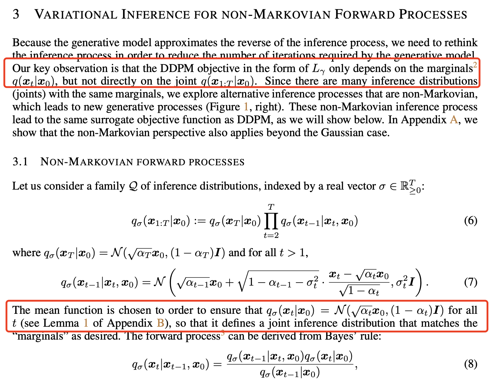
DENOISING DIFFUSION IMPLICIT MODELS,这个工作后面叫DDIM
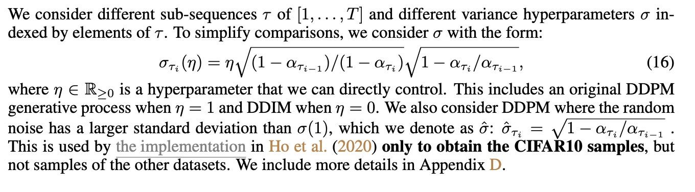
DDIM是把DDPM中马尔科夫假设(t-1的生成依赖于t)给去掉了,这样得到非马尔科夫假设的采样公式,可以跳步生成,采样过程大大加速。具体来说,作者通过构造均值函数的形式,使得qσ(xt∣xo)=N(αtx0,(1−αt)I)q_\sigma(x_t|x_o)=\mathcal{N}(\sqrt \alpha_t x_0, (1-\alpha_t)I)qσ(xt∣xo)=N(αtx0,(1−αt)I)的形式和DDPM中的形式是完全一样的,至于DDIM中的αt\alpha_tαt和DDPM中的αtˉ\bar{\alpha_t}αtˉ是一样的,这也是这篇论文刚上来看比较懵的一点,一个比较好的讲解可以参考【64、扩散模型加速采样算法DDIM论文精讲与PyTorch源码逐行解读-哔哩哔哩】 https://b23.tv/rhmEbo3
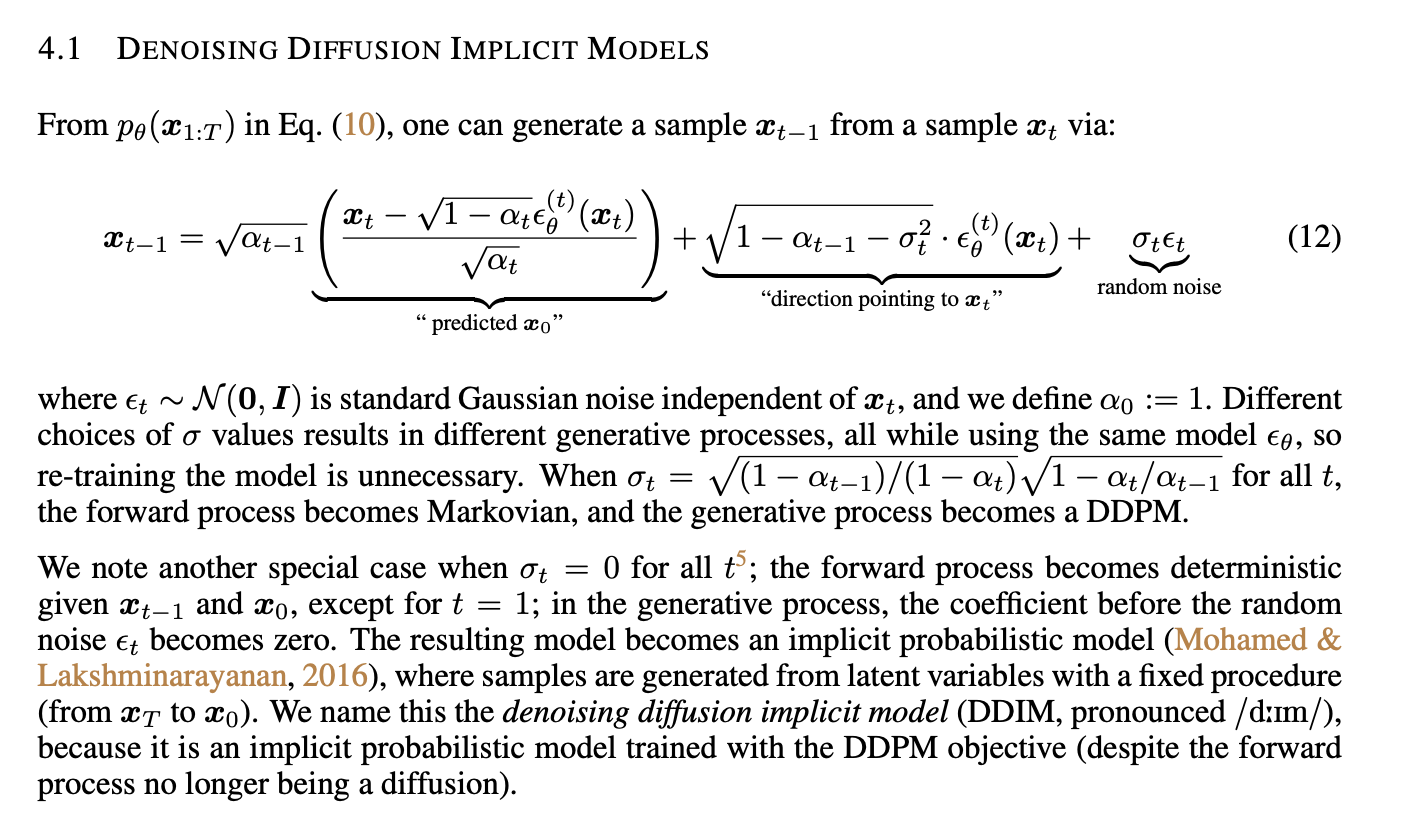
关于η\etaη的作用,η\etaη是一个超参数,η=1\eta=1η=1是原始DDMP,η=0\eta=0η=0是DDIP。
Diffusion Models Beat GANs on Image Synthesis
这也是发现DDPM在scale后效果后比较好OpenAI继续加大投入,这篇里面管自己的模型叫做ADM(ablated diffusion model):ADM refers to our ablated diffusion model, and ADM-G additionally uses classifier guidance;For upsampling, we use the upsampling stack from Nichol and Dhariwal [43] combined with our architecture improvements, which we refer to as ADM-U,几个要点:
- 模型变大变复杂,we match
BigGAN-deep even with as few as 25 forward passes per sample - Adaptive Group Normalization,We also experiment with a layer [43] that we refer to as adaptive group normalization (AdaGN), which incorporates the timestep and class embedding into each residual block after a group normalization operation [69], similar to adaptive instance norm [27] and FiLM [48].
- 这篇里面用了Classifier Guidance,Classifier Guidance的细节下面说
Classifier Guidance
Classifier Guidance这篇出现前diffusion model的在IS(Inception Score)和FID(Frechet lnception Distance)上的分数比不过GAN,Classifier Guidance的出现改变了这个局面,先来写写IS和FID的定义:
- IS(Inception Score):IS 实际上是在做一个 KL 散度计算,具体公式为
IS(G)=exp(Ex−pg(x)KL(p(y∣x)∣∣p(y)))IS(G)=exp(E_{x-p_g(x)}KL(p(y|x)||p(y)))IS(G)=exp(Ex−pg(x)KL(p(y∣x)∣∣p(y)))其中,p(y∣x)p(y|x)p(y∣x)是指对一张给定的生成图像x,将其输入预训练好的Inception-v3 分类网络后输出的类别概率,p(y)p(y)p(y)则是边缘分布,表示对于所有的生成图像来说,这个预训练好的分类网络输出的类别的概率的期望。如果生成图像中包含有意义且清晰可辨认的目标,则分类网络应该以很高的置信度将该图像判定为一个特定的类别,所以p(y∣x)p(y|x)p(y∣x)应该具有较小的。如果p(y)的熵较大,p(y|x)熵较小,即所生成的图像包含了非常多的类别,而每一张图像的类别又明确且置信度离,此时p(y|x)与p(y)的 KL 散度很大。可以看出,The original authors suggest using a sample of 50,000 generated images for this,IS并没有将真实样本与生成样本进行比较,它仅在量化生成样本的质量和多样性,IS分数越大越好。 - FID(Frechet lnception Distance):加入了真实样本与生成样本的比较它同样是将生成样本输入到分类网络中,不同的是,FID 不是对网络最后一层的输出概率P(y|x)进行操作,而是对网络倒数第二层的响应即特征图进行操作。具体来说,FID 是通过比较真实样本和生成样本的特征图的均值和方差来计算的,FID越小越好
- sFID: 在FID度量中增加spatial信息,除了标准FID引入的最后一层pooling之外,还额外引入了前边的7层conv的feature map来计算mean和covariance。
这里再补充一点Inception Score的核心code,code转载自https://github.com/sbarratt/inception-score-pytorch/tree/master
import torch
from torch import nn
from torch.autograd import Variable
from torch.nn import functional as F
import torch.utils.data

from torchvision.models.inception import inception_v3

import numpy as np
from scipy.stats import entropy

def inception_score(imgs, cuda=True, batch_size=32, resize=False, splits=1):
    """Computes the inception score of the generated images imgs

    imgs -- Torch dataset of (3xHxW) numpy images normalized in the range [-1, 1]
    cuda -- whether or not to run on GPU
    batch_size -- batch size for feeding into Inception v3
    splits -- number of splits
    """
    N = len(imgs)

    assert batch_size > 0
    assert N > batch_size

    # Set up dtype
    if cuda:
        dtype = torch.cuda.FloatTensor
    else:
        if torch.cuda.is_available():
            print("WARNING: You have a CUDA device, so you should probably set cuda=True")
        dtype = torch.FloatTensor

    # Set up dataloader
    dataloader = torch.utils.data.DataLoader(imgs, batch_size=batch_size)

    # Load inception model
    inception_model = inception_v3(pretrained=True, transform_input=False).type(dtype)
    inception_model.eval();
    up = nn.Upsample(size=(299, 299), mode='bilinear').type(dtype)
    def get_pred(x):
        if resize:
            x = up(x)
        x = inception_model(x)
        return F.softmax(x).data.cpu().numpy()

    # Get predictions
    preds = np.zeros((N, 1000))

    for i, batch in enumerate(dataloader, 0):
        batch = batch.type(dtype)
        batchv = Variable(batch)
        batch_size_i = batch.size()[0]

        preds[i*batch_size:i*batch_size + batch_size_i] = get_pred(batchv)

    # Now compute the mean kl-div
    split_scores = []

    for k in range(splits):
        part = preds[k * (N // splits): (k+1) * (N // splits), :]
        py = np.mean(part, axis=0)
        # py相当于求Inception Score的均值,也就是边缘概率P(y)
        scores = []
        for i in range(part.shape[0]):
            pyx = part[i, :] # pyx来自于Inception Score的向量,最后两个向量算KL
            scores.append(entropy(pyx, py))
        split_scores.append(np.exp(np.mean(scores)))
    return np.mean(split_scores), np.std(split_scores)

if __name__ == '__main__':
    class IgnoreLabelDataset(torch.utils.data.Dataset):
        def __init__(self, orig):
            self.orig = orig

        def __getitem__(self, index):
            return self.orig[index][0]

        def __len__(self):
            return len(self.orig)

    import torchvision.datasets as dset
    import torchvision.transforms as transforms

    cifar = dset.CIFAR10(root='data/', download=True,
                             transform=transforms.Compose([
                                 transforms.ToTensor(),
                                 transforms.Normalize((0.5, 0.5, 0.5), (0.5, 0.5, 0.5))
                             ])
    )

    IgnoreLabelDataset(cifar)

    print ("Calculating Inception Score...")
    print (inception_score(IgnoreLabelDataset(cifar), cuda=True, batch_size=32, resize=True, splits=10))
继续回到Classifier Guidance这个方法,这里其实是通过牺牲一部分图片的多样性来换取真实性。这里的guidance一般是一个在imagenet上预训练好的分类器,这个分类器的梯度刚好暗含了是否包含某类物体。Classifier Guidance通过引入预训练的分类器,利用贝叶斯定理将条件生成转化为无条件生成与分类器梯度的结合。数学上,条件生成的目标分数(score)可分解为无条件分数和分类器梯度项的加权和:
∇xtlogp(xt∣y)=∇xtlogp(xt)+s⋅∇xtlogp(y∣xt)\nabla_{x_t} \log p(x_t|y) = \nabla_{x_t} \log p(x_t) + s \cdot \nabla_{x_t} \log p(y|x_t)
∇xtlogp(xt∣y)=∇xtlogp(xt)+s⋅∇xtlogp(y∣xt)
其中,s(guidance scale)控制条件引导强度,logp(y∣xt)\log p(y|x_t)logp(y∣xt)是给定xtx_txt得到分类结果y,分类器需在带噪图像上训练。
CLASSIFIER-FREE DIFFUSION GUIDANCE
这篇的改进顾名思义,把Classifier Guidance里的Classifier通过有没有y:这里的y就表示guidance的信号,原来是个classifier,现在换成有这个文本就是y,没有这个文本就是空,来学这种距离。好处当然是摆脱了分类器限制,但缺点是有没有这个条件增加了forward的成本。原理是通过模型自身的有条件(条件输入)和无条件(条件随机丢弃)输出来构建引导信号,无需外部分类器。其核心公式为:
ϵCFG=ϵuncond+s⋅(ϵcond−ϵuncond)
\epsilon_{\text{CFG}} = \epsilon_{\text{uncond}} + s \cdot (\epsilon_{\text{cond}} - \epsilon_{\text{uncond}})
ϵCFG=ϵuncond+s⋅(ϵcond−ϵuncond)
其中,ϵcond\epsilon_{\text{cond}}ϵcond和ϵuncond\epsilon_{\text{uncond}}ϵuncond分别为有条件和无条件预测的噪声,s控制条件强度。

GLIDE (Guided Language to Image Diffusion for Generation and Editing)
Glide来自于GLIDE: Towards Photorealistic Image Generation and Editing with Text-Guided Diffusion Models这篇,有了上面那堆铺垫才能理解这篇,无非是把ADM改进成了Classifier Free Guidance,也就是摘要里提的 CLIP guidance and classifier-free guidance,重点关注下Guidance是怎么加进去的,直接看文中2.4部分即可:

文本经过transformer输出一组embedding后,进入ADM模型需要通过两条路径,一条是经过AdaGN进入ADM,另一条是进入concat到ADM的attention context中。这里的 f(xt)f(x_t)f(xt)是CLIP image encoder,g(c)g(c)g(c) 是CLIP text encoder。其中的 s 称作guidance scale(非常重要)。为什么对均值更新做改造就可以引入CLIP来guide,需要参考Diffusion Models Beat GANs on Image Synthesis的4.1章,需要一些公式推导,它的物理意义是在逐步采样过程中,多往caption和图像匹配值大的方向走,少往不一致的方向走。就这个物理意义而言,其实有很多别的实现方式。
DALL-E 2
- 基于 扩散模型(Diffusion Model):通过逐步去噪过程从随机噪声生成图像。
- 结合 CLIP 模型(Contrastive Language-Image Pretraining):CLIP 负责对齐文本和图像特征,指导扩散模型生成与文本匹配的内容。
- 分两阶段生成:首先生成低分辨率图像,再通过超分辨率模型提升细节。
Imagen
-
同样使用扩散模型,但更强调 大规模语言模型(如 T5-XXL) 的作用:通过预训练的文本编码器提取更精准的文本语义。
-
采用级联扩散模型:逐步生成从低到高分辨率的图像,每阶段细化细节(类似 DALL-E 2,但更依赖语言模型的文本理解能力)。
-
语言模型权重被冻结(仅用于文本编码),训练集中在图像生成部分。
Stable Diffusion原理
先上一个stable diffusion简易版的code镇楼:
def pipeline_forward(text: str, unet, vae) -> PIL.Image:
    latent = self.prepare_latent()
    prompt_embeds = self.text_encoder(text)
    for i, t in enumerate(self.timestamps):
        latents = torch.cat([latent]*2)
        noise_pred = unet(latents, t, prompt_embeds)
        noise_pred_uncond, noise_pred_text = noise_pred.chunk(2)
        noise_pred = noise_pred_uncond + self.guidance_scale * (noise_pred_text - noise_pred_uncond)
        noise_pred = rescale_noise_cfg(noise_pred,text) # 来自Common Diffusion Noise Schedules and Sample Steps are Flawed,把结束状态的信噪比降为0
        latent = self.scheduler.step(noise_pred, t, latent)
    image = vae.decode(latent)
    return image
再补一个简易版的unet code:
import torch
import torch.nn as nn
import torch.nn.functional as F

class UNet(nn.Module):
    def __init__(self, in_channels, out_channels):
        super(UNet, self).__init__()

        # 编码器部分
        self.encoder1 = self.double_conv(in_channels, 64)
        self.encoder2 = self.double_conv(64, 128)
        self.encoder3 = self.double_conv(128, 256)
        self.encoder4 = self.double_conv(256, 512)

        # 最底部的卷积
        self.bottleneck = self.double_conv(512, 1024)

        # 解码器部分
        self.upconv4 = self.upconv(1024, 512)
        self.decoder4 = self.double_conv(1024, 512)
        self.upconv3 = self.upconv(512, 256)
        self.decoder3 = self.double_conv(512, 256)
        self.upconv2 = self.upconv(256, 128)
        self.decoder2 = self.double_conv(256, 128)
        self.upconv1 = self.upconv(128, 64)
        self.decoder1 = self.double_conv(128, 64)

        # 最终的1x1卷积,用于生成分割图
        self.final_conv = nn.Conv2d(64, out_channels, kernel_size=1)

    def double_conv(self, in_channels, out_channels):
        """两次卷积操作"""
        return nn.Sequential(
            nn.Conv2d(in_channels, out_channels, kernel_size=3, padding=1),
            nn.BatchNorm2d(out_channels),
            nn.ReLU(inplace=True),
            nn.Conv2d(out_channels, out_channels, kernel_size=3, padding=1),
            nn.BatchNorm2d(out_channels),
            nn.ReLU(inplace=True)
        )

    def upconv(self, in_channels, out_channels):
        """上采样操作"""
        return nn.ConvTranspose2d(in_channels, out_channels, kernel_size=2, stride=2)

    def forward(self, x):
        # 编码器部分
        enc1 = self.encoder1(x)
        enc2 = self.encoder2(F.max_pool2d(enc1, kernel_size=2))
        enc3 = self.encoder3(F.max_pool2d(enc2, kernel_size=2))
        enc4 = self.encoder4(F.max_pool2d(enc3, kernel_size=2))

        # Bottleneck
        bottleneck = self.bottleneck(F.max_pool2d(enc4, kernel_size=2))

        # 解码器部分
        dec4 = self.upconv4(bottleneck)
        dec4 = torch.cat((dec4, self.crop_tensor(enc4, dec4)), dim=1)
        dec4 = self.decoder4(dec4)

        dec3 = self.upconv3(dec4)
        dec3 = torch.cat((dec3, self.crop_tensor(enc3, dec3)), dim=1)
        dec3 = self.decoder3(dec3)

        dec2 = self.upconv2(dec3)
        dec2 = torch.cat((dec2, self.crop_tensor(enc2, dec2)), dim=1)
        dec2 = self.decoder2(dec2)

        dec1 = self.upconv1(dec2)
        dec1 = torch.cat((dec1, self.crop_tensor(enc1, dec1)), dim=1)
        dec1 = self.decoder1(dec1)

        # 最后的1x1卷积生成输出
        return self.final_conv(dec1)

    def crop_tensor(self, encoder_tensor, decoder_tensor):
        """裁剪编码器张量,使其与解码器张量大小匹配"""
        _, _, H, W = decoder_tensor.size()
        encoder_tensor = self.center_crop(encoder_tensor, H, W)
        return encoder_tensor

    def center_crop(self, tensor, target_height, target_width):
        """中心裁剪函数"""
        _, _, h, w = tensor.size()
        crop_y = (h - target_height) // 2
        crop_x = (w - target_width) // 2
        return tensor[:, :, crop_y:crop_y + target_height, crop_x:crop_x + target_width]

# 使用示例
model = UNet(in_channels=1, out_channels=1)  # 输入和输出均为1通道(例如用于灰度图像)
input_image = torch.randn(1, 1, 572, 572)    # 随机生成一个输入图像
output = model(input_image)
print(output.shape)
来自于High-Resolution Image Synthesis with Latent Diffusion Models(https://ommer-lab.com/research/latent-diffusion-models/),Stable diffusion更像是商品名称,Latent diffusion更接近算法方案的描述,这俩说的是一个东西。

对于diffusion模型,在图像上的forward diffusion过程和reverse学习过程的计算量很大,而大部分的计算是花在了对于语义和感知影响不大的像素上。用在图像冗余信息的计算是可以被节省的。Latent diffusion模型的就是按照这个思路,先通过encoder来将图片变换到latent space,只保留语义信息,感知信息通过引入encoder/decoder来学习和压缩。即diffusion模型在stable diffusion中只处理低维的、强语义信息、低冗余的数据。对latent使用denoising diffusion模型来建模生成过程,并在denoising过程中通过attention机制引入用于指导生成内容的文本、图像等信息。整体目标函数如下图:

模型的实现包含了三个子模型,分别对应
- 图像像素空间到latent空间转化的AutoencoderKL
- latent空间中的Denoising UNetModel
- 引入文本prompt特征的FrozenOpenCLIPEmbedder
下面对代码进行一些分析
AutoencoderKL
使用https://huggingface.co/stabilityai/stable-diffusion-2的参数,对几个样例图像做encode和decode的结果,会发现decode后和原始图像非常接近。这部分代码在https://github.com/Stability-AI/stablediffusion/blob/main/ldm/models/autoencoder.py#L13
Denoising Unet
UNet中的prompt 特征的引入使用了cross attention,代码在https://github.com/Stability-AI/stablediffusion/blob/main/ldm/modules/diffusionmodules/openaimodel.py#L277。参考原文中的描述,y就是文本,KV就是文本学到的intermediate layers,用Q对应的UNet embedding来去找KV

Prompt的encoding
文中采用了ViT-H/14 on LAION-2B的embedding,文本的embedding tensor是高维的(77*1024),并没有清晰的图像语义信息,描述的语义相近的文本的embedding l2距离并不一定相近
Negative Prompt
回想一下,在文本到图像条件化中,提示被转换为嵌入向量,然后被输入到U-Net噪声预测器中。实际上有两组嵌入向量,一组用于正向提示,另一组用于负向提示。正向提示和负向提示地位平等。它们都有75个标记。你可以随时使用其中一个,或不使用另一个。负向提示是在采样器中通过classifier free guidance实现的,采样器负责实现反向差分。要理解负向提示的工作原理,我们首先需要理解在不使用负向提示的情况下采样是如何工作的。
更多可以参考https://zhuanlan.zhihu.com/p/644879268
ControlNet
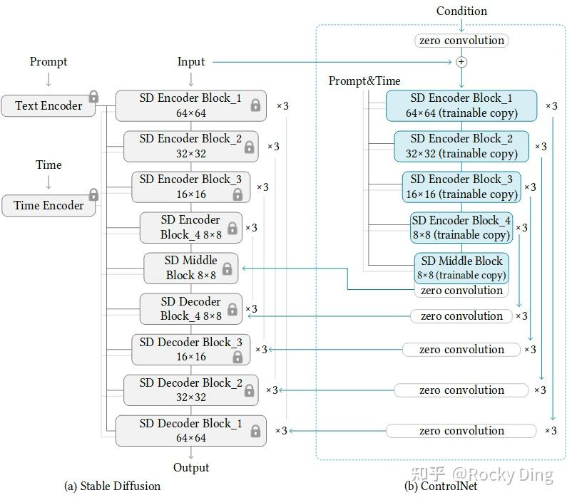
来自于Adding Conditional Control to Text-to-Image Diffusion Models,核心在于trainable copy前后各加一个zero convolution:

ControlNet模型的最小单元结构中有两个zero convolution模块,它们是1×1卷积,并且权重和偏置都初始化为零。这样一来,在我们开始训练ControlNet之前,所有zero convolution模块的输出都为零,使得ControlNet完完全全就在原有Stable Diffusion底模型的能力上进行微调训练,不会产生大的能力偏差。
controlnet什么模块和sd做交互?
在Stable Diffusion的U-Net中起作用,ControlNet主要将Stable Diffusion U-Net的Encoder部分和Middle部分进行复制训练,在Stable Diffusion U-Net的Decoder模块中通过skip connection加入了zero convolution模块处理后的特征,以实现对最终模型与训练数据的一致性。
如果zero convolution模块的初始权重为零,为什么zero convolution模块有效
这时很多人可能就会有一个疑问,如果zero convolution模块的初始权重为零,那么梯度也为零,ControlNet模型将不会学到任何东西。那么为什么“zero convolution模块”有效呢?(AIGC算法面试必考点)

Control Net在训练时,为什么会随机让50%的text prompt变为空?
促使模型更多的关注CfC_fCf,CfC_fCf是模型新加入的条件,是为了让模型学习用来控制图像生成。
DreamBooth
解决object fidelity的问题,生成图片和提供例子里的风格是一致的,不同于ControlNet针对细节的调整:

解决的思路是两点:
- 增加一些token id,通过lookup来找到高频、低频token的id
- 多样性是来自原来diffusion model的多样性。
最终使用dino距离来衡量效果
Text Inversion
-
嵌入空间扩展
Textual Inversion通过在模型的词嵌入空间中新增一个“伪词”(如S*)来表示目标概念。这个伪词对应的嵌入向量通过优化过程学习,使其能够捕捉目标概念的视觉特征。例如,用户提供多张宠物猫的照片,系统学习一个名为S_cat的伪词嵌入,使其在生成时能代表该猫的特征。 -
冻结模型参数
与DreamBooth等方法不同,Textual Inversion仅优化伪词的嵌入向量,而保持文本编码器(如CLIP)和生成模型(如UNet)的权重完全冻结。这使得训练成本极低(通常仅需几MB存储)。
部分摘自:
- https://mp.weixin.qq.com/s?__biz=MzkxMjYwOTIyMw==&mid=2247485934&idx=1&sn=222f9073d8559fbbc6b573131f781e0c&chksm=c061b04a638d50c3ccc41fc4e9c7527e626e09ae8be0bb17c05693c2c7e7ddc9292f09aeac3e#rd
- https://textual-inversion.github.io/
Stable Diffusion XL
以下转载自 https://huggingface.co/docs/diffusers/en/using-diffusers/sdxl,公众号有一篇解释比较详细的: https://mp.weixin.qq.com/s/3I0lFlRLonj-hD1bSQQD0Q
- the UNet is 3x larger and SDXL combines a second text encoder (OpenCLIP ViT-bigG/14) with the original text encoder to significantly increase the number of parameters
- introduces size and crop-conditioning to preserve training data from being discarded and gain more control over how a generated image should be cropped。其实就是在unet输入的参数中直接加了size和坐标的起点。size的参数叫做csizec_{size}csize,对应不同的分辨率,坐标的起点对应ccropc_{crop}ccrop这样就不会出现生成图片里熊猫头被裁掉的问题
- introduces a two-stage model process; the base model (can also be run as a standalone model) generates an image as an input to the refiner model which adds additional high-quality details
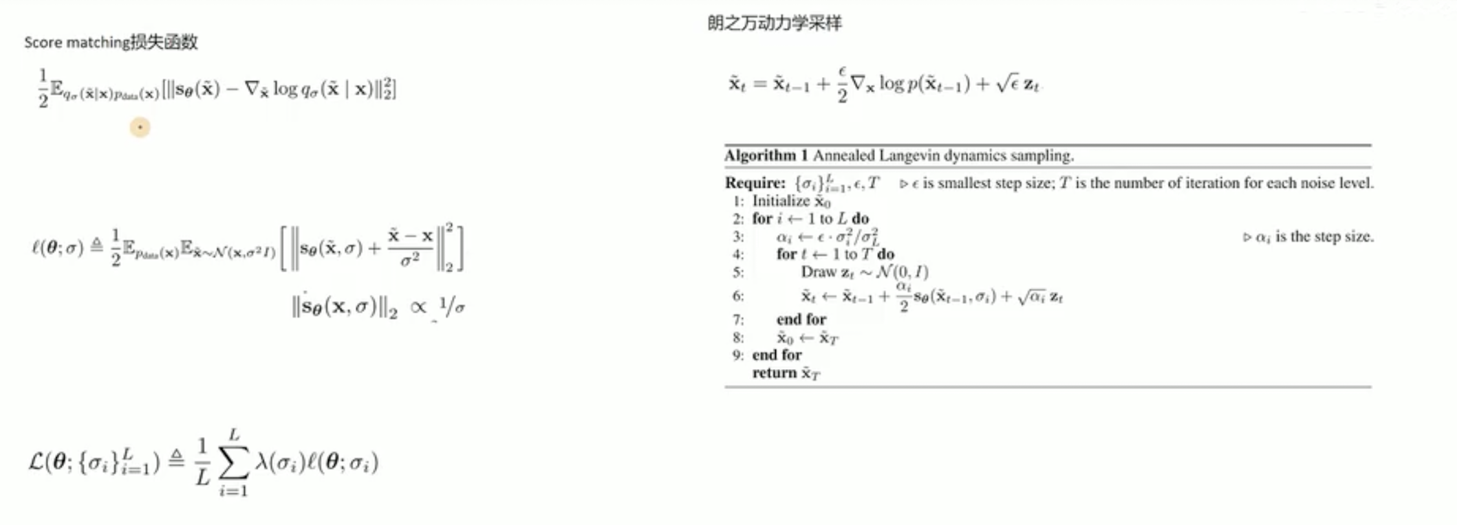
Score matching
score matching和diffusion model本质是同一个模型,score matching从score function角度建模,而diffusion model从贝叶斯角度建模,最终得到的loss非常相似,且sampling形式一致。从score function角度理解diffusion model的好处是很多SDE的现成工具可以引入进来,拓展出很多不同类型的diffusion model
朗之万蒙特卡洛采样(Langevin-MCMC)
推导可以参考视频【【AI知识分享】真正搞懂扩散模型Score Matching一定要理解的三大核心问题-哔哩哔哩】 https://b23.tv/N0Ucpox,下图截图来自来视频,视频中的推导想法大概还是从物理学粒子扩散的角度去推导:假设一滴墨水掉入整杯水发生扩散,朗之万蒙特卡洛采样利用布朗运动方程、玻尔兹曼分布建模了这个过程。
Denoising Score Matching
未详细看,来自于A Connection Between Score Matching and Denoising Autoencoders,大概的贡献是Score matching中的二阶导计算成本有点过高了,而denoising score matching方法可以降低成本做到
Noising Conditional Score Network(NCSN)
未详细看,来自于Generative Modeling by Estimating Gradients of the Data Distribution,大概的贡献是相当于从另一个角度解释了DDPM,给出了上面Aneled Langevin dynamics sampling的公式
Rectified flow
来自于Flow Straight and Fast: Learning to Generate and Transfer Data with Rectified Flow,原作者在知乎有一个较好的解读: https://zhuanlan.zhihu.com/p/603740431
DDPM的主要想法是不停叠加高斯噪声,反向过程可以看成是随机采样的高斯噪声x0经过flow得到一组生成图像x1的过程,但是这个flow基本是通过一系列Stochastic Differential Equation (SDE)偏微分方程利用Jessen不等式优化lower bound的过程,这个加噪、去噪过程比较慢作者认为flow过程走的不是直线
因此Rectified flow就是利用走直线把原来不是直线的flow过程变成直线给加速了,优化目标参考下图
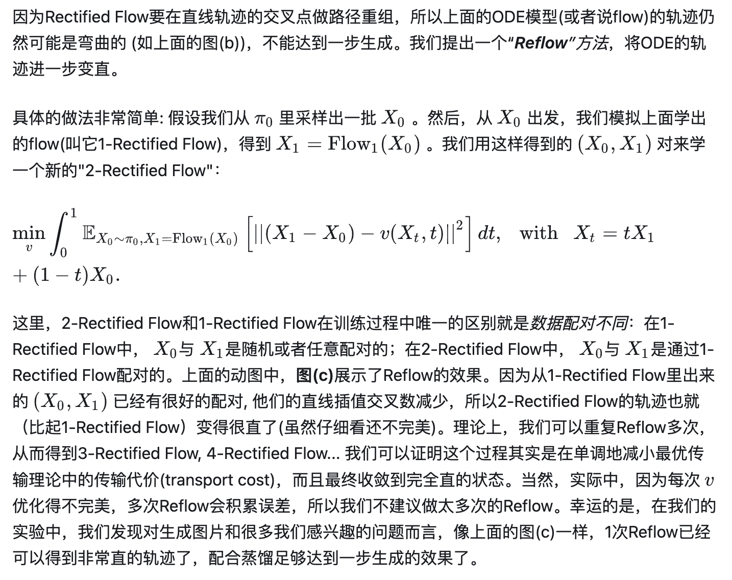
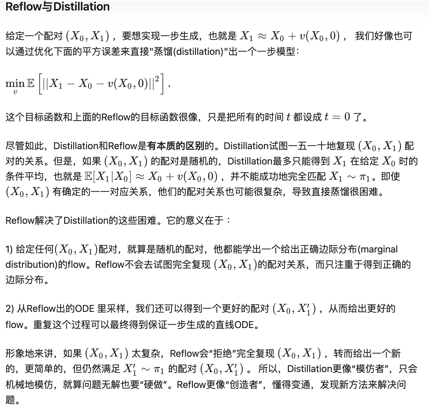
Rectified flow可以看成是一个二分图匹配的问题,Reflow和蒸馏的区别仅在于是否对传输的路径v进行刻画:
Stable Diffusion 3
来自Scaling Rectified Flow Transformers for High-Resolution Image Synthesis这篇文章,主要有以下几个贡献
Tailored SNR Samplers for RF models
rectified flow model 在训练时针对所有的 timestep 是均匀采样的,一个假设是在中间的 timestep 会比两边的更难学,因此对不同位置的 t 乘以不同的权重,作者讨论了几种方案用的是CosMap
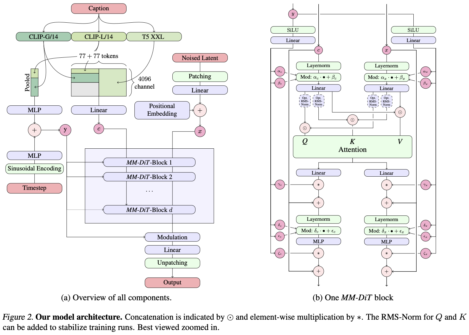
模型结构
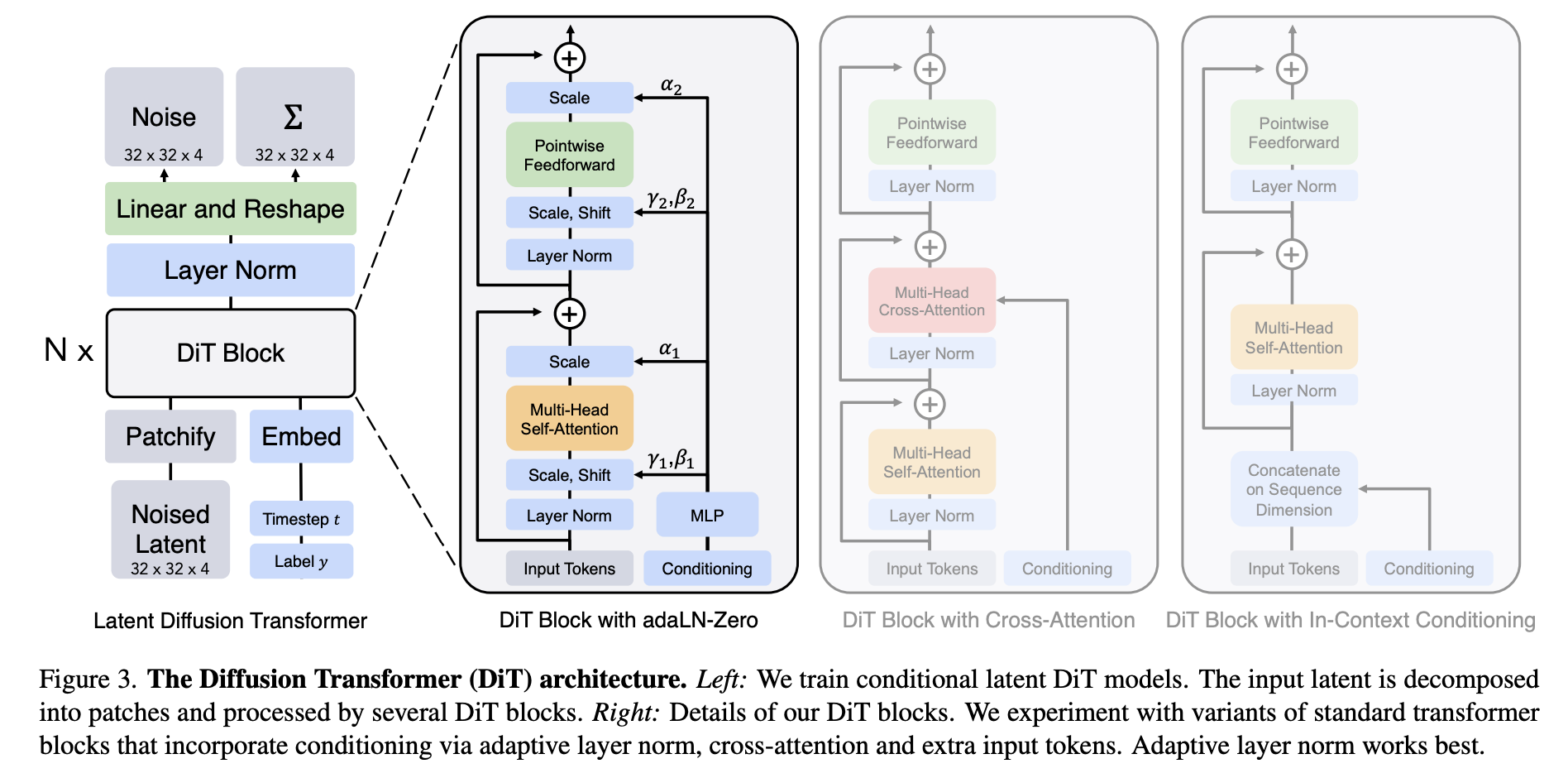
模型结构用了MMDiT,是DiT的一个升级版,就是MultiModality这么直白的意思,参考下面MM-DiT Block:
- Adaptive layer norm (adaLN) condition:将ViT block中的LayerNorm改造成adaLayerNorm,不是直接学习LayerNorm中的γ\gammaγ,β\betaβ,而是用所有条件信息 embedding的sum作为输入,以逻辑回归的形式来预测这两个值,建模逻辑回归问题也是使用的神经网络,一个简单的MLP层,这种condition方式引入的开销最小,在diffusers/models/transformers/transformer_sd3.py中叫做AdaLayerNormContinuous
- adaLN-Zero block. Prior work on ResNets has found that initializing each residual block as the identity function is beneficial.在diffusers/models/transformers/transformer_sd3.py中叫做AdaLayerNormZero。把 residual block 初始化为恒等函数比较好(即输入直接输出),因此在残差前加一个 scale 参数,也是 t 和 c 回归学到的,并且初始化 MLP 使这个参数为 0 ,向量
- 输入可以看下面代码,同样摘自上面路径,hidden_states是图像的Noised Latent,encoder_hidden_states是condition,一般也就是kv,名字里带着encoder这俩分别和时间的temb过norm(这个embed就是用transformer中sin cos思路得到的),norm后再过msa
        norm_hidden_states, gate_msa, shift_mlp, scale_mlp, gate_mlp = self.norm1(hidden_states, emb=temb)

        if self.context_pre_only:
            norm_encoder_hidden_states = self.norm1_context(encoder_hidden_states, temb)
        else:
            norm_encoder_hidden_states, c_gate_msa, c_shift_mlp, c_scale_mlp, c_gate_mlp = self.norm1_context(
                encoder_hidden_states, emb=temb
            )
        # Attention.
        attn_output, context_attn_output = self.attn(
            hidden_states=norm_hidden_states, encoder_hidden_states=norm_encoder_hidden_states
        )
Dit是把class label 作为 conditional input
笔记参考了以下信息
- 【DALL·E 2(内含扩散模型介绍)【论文精读】】https://www.bilibili.com/video/BV17r4y1u77B?vd_source=e260233b721e72ff23328d5f4188b304
- https://kexue.fm/archives/9119
- Denoising Diffusion Probabilistic Models
- Improved Denoising Diffusion Probabilistic Models
- Hulu书
- GLIDE: Towards Photorealistic Image Generation and Editing with Text-Guided Diffusion Models
- Stable Diffusion:High-Resolution Image Synthesis with Latent Diffusion Models
- 深入浅出完整解析ControlNet核心基础知识 https://zhuanlan.zhihu.com/p/660924126


 被折叠的 条评论
为什么被折叠?
被折叠的 条评论
为什么被折叠?
 到【灌水乐园】发言


