


kNN (k-nearest neighbor)的定义
针对一个测试实例,在给定训练集中,基于某种距离度量找到与之最近的k个实例点,然后基于这k个最邻近实例点的信息,以某种决策规则来对该测试实例进行分类或回归。
由定义可知, k N N kNN kNN模型包含三个基本要素:距离度量、k值选择以及决策规则。再详细描述这三要素之前,我们先用一个样图来简单描述 k N N kNN kNN分类模型的效果。
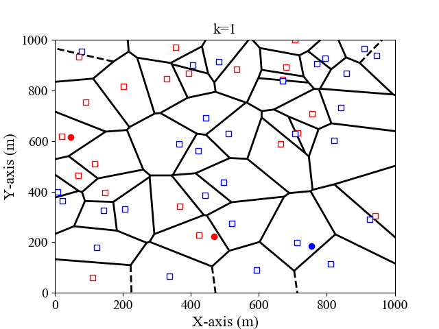
我们以二维平面为例,假设输入的训练集格式为 ( x 1 , x 2 , l ) (x_1,x_2,l) (x1,x2,l),其中 x 1 , x 2 x_1, x_2 x1,x2为横纵坐标, l l l为标签。这里我们考虑 k = 1 , 3 k=1,3 k=1,3的情况,决策规则为多数投票规则,即测试实例与k个实例中的多数属于同一类。图 1 , 2 1,2 1,2分别是 k = 1 , 3 k=1,3 k=1,3时,二维特征空间划分图。
距离度量
k N N kNN kNN的本质是“近朱者赤近墨者黑”,即测试点的类别由其最邻近的 k k k个实例点决定。这里“最邻近”的意义根据距离度量的不同而不同。一般来说,我们最常见的便是欧氏距离。这里我们介绍包含欧氏距离,但比欧氏距离更普适的Minkowski距离。
假定训练集中,每个实例包含 n n n个特征,那么实例 x x x可以分别表示为 x = ( x 1 , ⋯ , x n ) x=(x_1,\cdots,x_n) x=(x1,⋯,xn)。假定测试实例为 y = ( y 1 , ⋯ , y n ) y=(y_1,\cdots,y_n) y=(y1,⋯,yn),那么 x , y x, y x,y之间的Minkowski距离可以表示为:
L ( x , y ) = ( ∑ i = 1 n ∣ x i − y i ∣ p ) 1 p , L(x,y)=\left(\sum\limits_{i=1}^{n}{\lvert x_i-y_i\rvert}^p\right)^{\frac{1}{p}}, L(x,y)=(i=1∑n∣xi−yi∣p)p1,
其中,
p
>
0
p>0
p>0是一个可变参数:
L
(
x
,
y
)
=
{
∑
i
=
1
n
∣
x
i
−
y
i
∣
,
p
=
1
(曼哈顿距离)
(
∑
i
=
1
n
∣
x
i
−
y
i
∣
2
)
1
2
,
p
=
2
(欧氏距离)
max
i
=
1
n
∣
x
i
−
y
i
∣
,
p
→
∞
,
(切比雪夫距离)
L(x,y)= \begin{cases} \sum\limits_{i=1}^{n}{\lvert x_i-y_i\rvert},\quad p=1\quad\text{(曼哈顿距离)}\\ \left(\sum\limits_{i=1}^{n}{\lvert x_i-y_i\rvert}^2\right)^{\frac{1}{2}},\quad p=2\quad\text{(欧氏距离)}\\ \max\limits_{i=1}^{n}{\lvert x_i-y_i\rvert},\quad p\to\infty,\quad\text{(切比雪夫距离)} \end{cases}
L(x,y)=⎩⎪⎪⎪⎪⎪⎨⎪⎪⎪⎪⎪⎧i=1∑n∣xi−yi∣,p=1(曼哈顿距离)(i=1∑n∣xi−yi∣2)21,p=2(欧氏距离)i=1maxn∣xi−yi∣,p→∞,(切比雪夫距离)
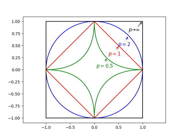
当然
p
p
p也可以取小于
1
1
1的值,如
p
=
1
2
p=\frac{1}{2}
p=21。图
3
3
3给出了当
p
p
p取不同值时,与原点距离为
1
1
1的图形:
k k k值的选择
调参是机器学习算法的重要一环。在 k N N kNN kNN算法中, k k k值的选取对结果的影响较大。下面以图 4 4 4来距离说明:
(a)当
k
k
k取值较小时,此时是根据测试实例周围较少的训练样例信息来进行分类。由于训练样例离测试样例比较近,因此训练误差比较小。当这些邻近的训练样例是噪声时,会严重影响分类结果,即泛化误差变大。
(b)当
k
k
k取值较大时,此时是根据测试实例周围较多的训练样例信息来进行分类。这时与测试实例相距较远(相关性较小)的训练样例也对分类结果有影响,使得泛化误差较大。一个极端的例子就是以考虑所有的训练样例,这时测试样例被归为训练样例数最大的一类。
Note: 模型复杂度的理解:对于有参模型来说(例如线性拟合),模型复杂度一般可以用参数的多少来判断。对于无参模型来说(例如这里的 k N N kNN kNN),这里还需思考。可能的情况?考虑极端情况,当 k k k取值为整个训练样例数时,这时的模型最简单,即测试样例被归为训练样例数最大的一类。当 k k k取值为 1 1 1时,每个测试样例都需要根据其最邻近节点来进行分类,这时模型变得很复杂。
通常来说,我们可以通过交叉验证来选取 k k k值。同时,我们也可以对这 k k k个训练样例进行距离加权,来克服(b)的影响。
决策规则
k N N kNN kNN既可进行分类,也可用于回归。
- 对于分类问题来说,一般采用的是投票法,即测试样例被归为最邻近 k k k个训练样例数中最大的一类。
- 对于回归问题来说,一般采用的是平均法。顾名思义,测试样例的取值为这 k k k个训练样例取值的平均值。
- 最后,我们可以对这两种方法进行改进,即对这 k k k个训练样例进行加权,离测试样例较近的训练样例一般具有更大的影响权重。
k N N kNN kNN优缺点:
优点:
最近更新于20-01-20,明早就回家过年了,年后再更新。
未完待续。。。
最近更新于20-03-30,优缺点还需用图示说明。
算法实践
下面我们给出两种方式实现KNN分类算法:一、自己编程实现KNN算法;二、使用更加简单的scikit-learn库。
注意:数据集为iris数据集,有150个训练集,4个feature, 总共分3类。在方法一中,我们考虑了所有4个feature,将所有150个训练数据作为训练(即在程序中设置split=1),读者可以通过设置split的值来获取测试集用于交叉检验得到最佳的k值。在方法二中,我们只考虑了前2个feature,这么做是为了在二维图中展示分类结果。
自写KNN算法
- 算法思路:
- 计算已知数据集中的点与当前点之间的距离
- 按照距离递增次序进行排序
- 选取与当前点距离最小的K个点
- 确定这K个点所在类别的出现次数
- 返回这K个点出现次数最多的类别作为当前点的预测分类
- 代码实现
from sklearn import datasets, neighbors
import random
import math
import numpy as np

# Divide the original dataset into training data and test data
def LoadDataSet(irisData, split, trainData, testData, trainLabel, testLabel):
    allData = irisData.data
    allLabel = irisData.target
    for i in range(len(allData)):
        if random.random() < split:  #
            trainData.append(allData[i])
            trainLabel.append(allLabel[i])
        else:
            testData.append(allData[i])
            testLabel.append(allLabel[i])

# Calculate the distance between two instance
def CalDist(instance1, instance2):
    dist = 0
    length = len(instance1)
    for i in range(length):
        dist += pow((instance1[i] - instance2[i]), 2)
    return math.sqrt(dist)

# The KNN algorithm
def knn(instance, k, trainData, trainLabel):
    allDist = []
    # Calculate distances from all training data
    for i in range(len(trainData)):
        allDist.append([CalDist(instance, trainData[i]), i])
    allDist.sort()
    # Determine the neighbors
    neighbors = []
    for j in range(k):
        neighbors.append(allDist[j][1])
    numLabels = len(np.unique(trainLabel))
    vote = [0] * numLabels
    # Vote to decide the resultant label
    for kk in range(k):
        vote[trainLabel[neighbors[kk]]] += 1
    # print the result
    print(vote.index(max(vote)))

# load dataset of iris
irisData = datasets.load_iris()

# All data are used for training
split = 1
# Number of neighbors
k = 3
trainData = []
trainLabel = []
testData = []
testLabel = []
LoadDataSet(irisData, split, trainData, testData, trainLabel, testLabel)

predictPoint=[7.6, 3., 6.6, 2.1]

knn(predictPoint, k, trainData, trainLabel)
使用scikit-learn库
- 代码实现
import numpy as np
import matplotlib.pyplot as plt
from matplotlib.colors import ListedColormap
from sklearn import neighbors, datasets

# The number of neighbors
k = 3

# import dataset of iris
iris = datasets.load_iris()

# The first two-dim feature for simplicity
X = iris.data[:, :2]
# The labels
y = iris.target

h = .02  # step size in the mesh

# Create color maps for three types of labels
cmap_light = ListedColormap(['tomato', 'limegreen', 'cornflowerblue'])

# we create an instance of Neighbours Classifier and fit the data.
clf = neighbors.KNeighborsClassifier(k, 'uniform')
clf.fit(X, y)

# Plot the decision boundary. Assign a color to each point in the mesh.
x_min, x_max = X[:, 0].min() - 1, X[:, 0].max() + 1
y_min, y_max = X[:, 1].min() - 1, X[:, 1].max() + 1
xx, yy = np.meshgrid(np.arange(x_min, x_max, h),
                     np.arange(y_min, y_max, h))
Z = clf.predict(np.c_[xx.ravel(), yy.ravel()])

# Z is a matrix (values) for the two-dim space
Z = Z.reshape(xx.shape)


# Plot the training points: different
def PlotTrainPoint():
    for i in range(0, len(X)):
        if y[i] == 0:
            plt.plot(X[i][0], X[i][1], 'rs', markersize=6, markerfacecolor="r")
        elif y[i] == 1:
            plt.plot(X[i][0], X[i][1], 'gs', markersize=6, markerfacecolor="g")
        else:
            plt.plot(X[i][0], X[i][1], 'bs', markersize=6, markerfacecolor="b")


# Set the format of labels
def LabelFormat(plt):
    ax = plt.gca()
    plt.tick_params(labelsize=14)
    labels = ax.get_xticklabels() + ax.get_yticklabels()
    [label.set_fontname('Times New Roman') for label in labels]
    font1 = {'family': 'Times New Roman',
             'weight': 'normal',
             'size': 16,
             }


# Plot the boundary lines (contour figure)
fig = plt.figure()
plt.contour(xx, yy, Z, 3, colors='black', linewidths=1, linestyles='solid')
PlotTrainPoint()
plt.title("3-Class classification (k = %i, weights = '%s')" % (k, 'uniform'), LabelFormat(plt))
plt.show()

# Plot the boundary maps (mesh figure)
plt.figure()
plt.pcolormesh(xx, yy, Z, cmap=cmap_light)
PlotTrainPoint()
plt.xlim(xx.min(), xx.max())
plt.ylim(yy.min(), yy.max())
plt.title("3-Class classification (k = %i, weights = '%s')" % (k, 'uniform'), LabelFormat(plt))
plt.show()
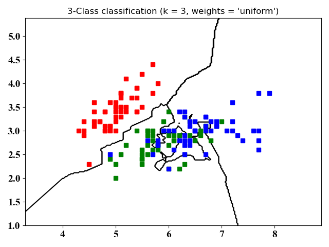
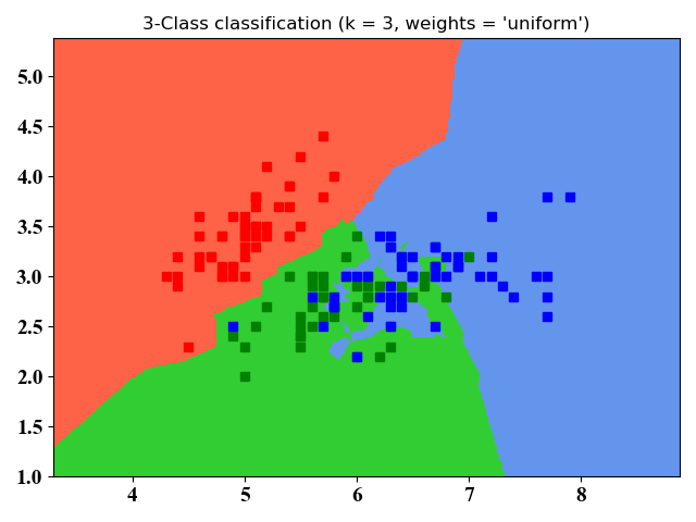
- 仿真结果
图4和图5没有本质区别,不同之处在于图4只画了分类的轮廓,图5是将整个空间的点进行了分类。从图中可以看出,kNN适合于非线性分类。
附录
图1的python 源代码:
import numpy as np
import matplotlib.pyplot as plt
import matplotlib as mpl
from scipy.spatial import Voronoi, voronoi_plot_2d, cKDTree
import pickle

# The number of test points and train points
Num_test = 3
Num_train = 50
# Generate the two-dimension feature (x,y), Here x,y are coordinates
Loc_x_train = 1000 * np.random.rand(Num_train, 1)
Loc_y_train = 1000 * np.random.rand(Num_train, 1)
Label_train = np.round(np.random.rand(Num_train, 1))
Loc_train = 1000 * np.random.rand(Num_train, 2)
filename = 'Loc_x_train'

# Generate the test points
Loc_x_test = 1000 * np.random.rand(Num_test, 1)
Loc_y_test = 1000 * np.random.rand(Num_test, 1)
Loc_test = 1000 * np.random.rand(Num_test, 2)

for i in range(0, len(Loc_x_train)):
    Loc_train[i] = [Loc_x_train[i], Loc_y_train[i]]
for i in range(0, len(Loc_x_test)):
    Loc_test[i] = [Loc_x_test[i], Loc_y_test[i]]

# Use the scipy.spatial packets to form voronoi
vor = Voronoi(Loc_train)
fig = voronoi_plot_2d(vor, show_points=False, show_vertices=False,
                      line_colors='black', line_width=2, line_alpha=1,
                      point_size=15)
# Plot the train pints
for i in range(0, Num_train):
    if Label_train[i]:
        plt.plot(Loc_x_train[i], Loc_y_train[i], 'rs', markersize=6, markerfacecolor="w")
    else:
        plt.plot(Loc_x_train[i], Loc_y_train[i], 'bs', markersize=6, markerfacecolor="w")

# Use the kdtree to find the nearest train point for each test point
voronoi_kdtree = cKDTree(Loc_train)
test_point_dist, test_point_regions = voronoi_kdtree.query(Loc_test)

# Classify the test points, the same color as the nearest train point
for i in range(0, Num_test):
    if Label_train[test_point_regions[i]]:
        plt.plot(Loc_x_test[i], Loc_y_test[i], 'ro', markersize=6)
    else:
        plt.plot(Loc_x_test[i], Loc_y_test[i], 'bo', markersize=6)

# The following are typical settings for plotting figures
plt.axis([0, 1001, 0, 1001])
ax = plt.gca()
plt.tick_params(labelsize=14)
labels = ax.get_xticklabels() + ax.get_yticklabels()
[label.set_fontname('Times New Roman') for label in labels]
font1 = {'family': 'Times New Roman',
         'weight': 'normal',
         'size': 16,
         }

plt.xlabel('X-axis (m)', font1)
plt.ylabel('Y-axis (m)', font1)
plt.title('k=1', font1)
plt.savefig('f2.png')
plt.show()
图3的python源代码:
import numpy as np
import matplotlib.pyplot as plt
import matplotlib as mpl
from scipy.spatial import Voronoi, voronoi_plot_2d, cKDTree
import pickle
import math


original_point = [0, 0]

x = np.linspace(-1, 1, 10000)

# p=0.5
y1 = 1 + np.abs(x) - 2 * np.power(np.abs(x), 0.5)
y2 = - y1
plt.plot(x, y1, 'g')
plt.plot(x, y2, 'g')
# p=1
y1 = 1 - np.abs(x)
y2 = np.abs(x) - 1
plt.plot(x, y1, 'r')
plt.plot(x, y2, 'r')
# p=2
y1 = np.power(1 - np.power(x, 2), 1 / 2)
y2 = -y1
plt.plot(x, y1, 'b-')
plt.plot(x, y2, 'b-')

# p-> infty
for i in range(0, len(x)):
    if np.abs(x[i]) == 1:
        y1[i] = 0
    else:
        y1[i] = 1
y2 = -y1
plt.plot(x, y1, 'k-')
plt.plot(x, y2, 'k-')


# To plot figures
plt.axis('equal')
ax=plt.gca()

plt.annotate('$p=0.5$', xy=(0.25, 0.25), xycoords='data',
             xytext=(-25, -25), textcoords='offset points', color='g', fontsize=12, arrowprops=dict(arrowstyle="->",
             connectionstyle="arc,rad=0", color='g'))
plt.annotate('$p=1$', xy=(0.5, 0.5), xycoords='data',
             xytext=(-25, -25), textcoords='offset points', color='r', fontsize=12, arrowprops=dict(arrowstyle="->",
             connectionstyle="arc,rad=0", color='r'))
plt.annotate('$p=2$', xy=(0.7, 0.7), xycoords='data',
             xytext=(-25, -25), textcoords='offset points', color='b', fontsize=12, arrowprops=dict(arrowstyle="->",
             connectionstyle="arc,rad=0", color='b'))
plt.annotate(r'$p\to\infty$', xy=(1, 1), xycoords='data',
             xytext=(-35, -25), textcoords='offset points', color='k', fontsize=12, arrowprops=dict(arrowstyle="->",
             connectionstyle="arc,rad=0", color='k'))

plt.savefig('f3.png')
plt.show()


 3102
3102

 被折叠的 条评论
为什么被折叠?
被折叠的 条评论
为什么被折叠?
 到【灌水乐园】发言


