


loss_layer:
AccuracyLayer类;
LossLayer类;
ContrastiveLossLayer类;
EuclideanLossLayer类;
HingeLossLayer类;
InfogainLossLayer类;
MultinomialLogisticLossLayer类;
SigmoidCrossEntropyLossLayer类;
SoftmaxWithLossLayer类;
终于看到最后一层了。
首先定义了一个常数:
const float kLOG_THRESHOLD = 1e-20;
1 AccuracyLayer:
Computes the classification accuracy for a one-of-many classification task.
1.1 原理介绍:
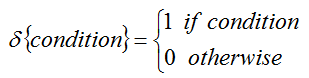
首先需要弄清楚,这个层是什么作用,上面的粉红色字体告诉我们,该层是计算分类精度的。所以我们常常在论文中会看到top-1, top5就是这里计算出来的。
假设批量训练的时候,一个批量的大小是N,那么对该批量的训练精度可以表示为:
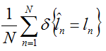
其中:
分类标签的预测值为:

分类标签的实际值为:

那么top-1也就是将评分最高的那个预测分类标签与实际标签做比较,而top-5是将评分最高的前5个预测分类标签与实际标签做比较(只要有一个比较成功就算是成功)。
由于只是计算精度,所以没有反馈。
另外还可以推出,这个层通常处于最末端。
1.2 属性变量:
int top_k_;这个变量在前面已经介绍过了。
1.3 构造函数:
template <typename Dtype>
void AccuracyLayer<Dtype>::LayerSetUp(
  const vector<Blob<Dtype>*>& bottom, vector<Blob<Dtype>*>* top) {
  top_k_ = this->layer_param_.accuracy_param().top_k();
}

template <typename Dtype>
void AccuracyLayer<Dtype>::Reshape(
  const vector<Blob<Dtype>*>& bottom, vector<Blob<Dtype>*>* top) {
  CHECK_EQ(bottom[0]->num(), bottom[1]->num())
      << "The data and label should have the same number.";
  CHECK_LE(top_k_, bottom[0]->count() / bottom[0]->num())
      << "top_k must be less than or equal to the number of classes.";
  CHECK_EQ(bottom[1]->channels(), 1);
  CHECK_EQ(bottom[1]->height(), 1);
  CHECK_EQ(bottom[1]->width(), 1);
  (*top)[0]->Reshape(1, 1, 1, 1);
}
从 LayerSetUp()中可以看到,top_k是可以在网络配置文件中设置的。
另外,因为该层的目的只是计算精度,所以top层只有1个元素。
1.4 前馈函数:
template <typename Dtype>
void AccuracyLayer<Dtype>::Forward_cpu(const vector<Blob<Dtype>*>& bottom,
    vector<Blob<Dtype>*>* top) {
  Dtype accuracy = 0;
  const Dtype* bottom_data = bottom[0]->cpu_data();
  const Dtype* bottom_label = bottom[1]->cpu_data();
  int num = bottom[0]->num();
  int dim = bottom[0]->count() / bottom[0]->num();
  vector<Dtype> maxval(top_k_+1);
  vector<int> max_id(top_k_+1);
  for (int i = 0; i < num; ++i) {
    // Top-k accuracy
    std::vector<std::pair<Dtype, int> > bottom_data_vector;
    for (int j = 0; j < dim; ++j) {
      bottom_data_vector.push_back(
          std::make_pair(bottom_data[i * dim + j], j));
    }
    std::partial_sort(
        bottom_data_vector.begin(), bottom_data_vector.begin() + top_k_,
        bottom_data_vector.end(), std::greater<std::pair<Dtype, int> >());
    // check if true label is in top k predictions
    for (int k = 0; k < top_k_; k++) {
      if (bottom_data_vector[k].second == static_cast<int>(bottom_label[i])) {
        ++accuracy;
        break;
      }
    }
  }

  // LOG(INFO) << "Accuracy: " << accuracy;
  (*top)[0]->mutable_cpu_data()[0] = accuracy / num;
  // Accuracy layer should not be used as a loss function.
}
整个过程不难理解,其中用到了比较有意思的 部分排序——partial_sort,然后其中定义的max_id似乎没有用的样子欸。
2 LossLayer:
An interface for Layer%s that take two Blob%s as input -- usually (1) predictions and (2) ground-truth labels -- and output a singleton Blob representing the loss.
LossLayers are typically only capable of backpropagating to their first input -- the predictions.
这里就先不介绍了,因为从类中可以看到,这还只是一个抽象类,说明在caffe中实现了各种损失层,都继承了这个抽象类:
template <typename Dtype>
class LossLayer : public Layer<Dtype> {
 public:
  explicit LossLayer(const LayerParameter& param)
     : Layer<Dtype>(param) {}
  virtual void LayerSetUp(
      const vector<Blob<Dtype>*>& bottom, vector<Blob<Dtype>*>* top);
  virtual void Reshape(
      const vector<Blob<Dtype>*>& bottom, vector<Blob<Dtype>*>* top);

  virtual inline int ExactNumBottomBlobs() const { return 2; }

  /**
   * @brief For convenience and backwards compatibility, instruct the Net to
   *        automatically allocate a single top Blob for LossLayers, into which
   *        they output their singleton loss, (even if the user didn't specify
   *        one in the prototxt, etc.).
   */
  virtual inline bool AutoTopBlobs() const { return true; }
  virtual inline int ExactNumTopBlobs() const { return 1; }
  /**
   * We usually cannot backpropagate to the labels; ignore force_backward for
   * these inputs.
   */
  virtual inline bool AllowForceBackward(const int bottom_index) const {
    return bottom_index != 1;
  }
};
3 ContrastiveLossLayer:
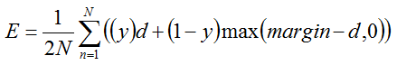
Computes the contrastive loss
where
This can be used to train siamese networks.
@param bottom input Blob vector (length 3)
-# @f$ (N \times C \times 1 \times 1) @f$
the features:
-# @f$ (N \times C \times 1 \times 1) @f$
the features:
-# @f$ (N \times 1 \times 1 \times 1) @f$
the binary similarity:

3.1 原理介绍:
这是一种损失值计算方式,上面也提到了,这种损失值对于siamese network很有用,这种网络是05年Yann Lecun提出来的,它的特点是它接收两个图片作为输入,而不是一张图片作为输入。
摘抄自caffe github的issue697
Siamese nets are supervised models for metric learning [1].
[1] S. Chopra, R. Hadsell, and Y. LeCun. Learning a similarity metric discriminatively, with application to face verification. In Computer Vision and Pattern Recognition, 2005. CVPR 2005. IEEE Computer Society Conference on, volume 1, pages 539–546. IEEE, 2005. http://yann.lecun.com/exdb/publis/pdf/chopra-05.pdf
Speaking of metric learning, I remember that @norouzi had proposed and open sourced a method that learned a Hamming distance metric to distinguish similar and dissimilar images [2].
[2] Mohammad Norouzi, David J. Fleet, Ruslan Salakhutdinov, Hamming Distance Metric Learning, Neural Information Processing Systems (NIPS), 2012.
根据前面的介绍,其实该层的前馈计算过程已经算是描述清楚了,那么反馈过程是怎样的呢?
根据链式法则有:
当两图相似的时候(也就是y=1):
对b的求导也就是多了一个负号而已。
当两图不相似时(也就是y=0):
因为margin是常量,所以求导过程与上面类似,只是还要再多一个负号。当然这里面还要分margin-d是否大于0,如果小于0,导数还是0。
3.2 属性变量:
  Blob<Dtype> diff_;  // cached for backward pass
  Blob<Dtype> dist_sq_;  // cached for backward pass
  Blob<Dtype> diff_sq_;  // tmp storage for gpu forward pass
  Blob<Dtype> summer_vec_;  // tmp storage for gpu forward pass
3.3 构造函数:
template <typename Dtype>
void ContrastiveLossLayer<Dtype>::LayerSetUp(
  const vector<Blob<Dtype>*>& bottom, vector<Blob<Dtype>*>* top) {
  LossLayer<Dtype>::LayerSetUp(bottom, top);
  CHECK_EQ(bottom[0]->channels(), bottom[1]->channels());
  CHECK_EQ(bottom[0]->height(), 1);
  CHECK_EQ(bottom[0]->width(), 1);
  CHECK_EQ(bottom[1]->height(), 1);
  CHECK_EQ(bottom[1]->width(), 1);
  CHECK_EQ(bottom[2]->channels(), 1);
  CHECK_EQ(bottom[2]->height(), 1);
  CHECK_EQ(bottom[2]->width(), 1);
  diff_.Reshape(bottom[0]->num(), bottom[0]->channels(), 1, 1);
  diff_sq_.Reshape(bottom[0]->num(), bottom[0]->channels(), 1, 1);
  dist_sq_.Reshape(bottom[0]->num(), 1, 1, 1);
  // vector of ones used to sum along channels
  summer_vec_.Reshape(bottom[0]->channels(), 1, 1, 1);
  for (int i = 0; i < bottom[0]->channels(); ++i)
    summer_vec_.mutable_cpu_data()[i] = Dtype(1);
}
前面说到这种siamese network的输入是两个图片,那么为啥这里在检测底层Blob的时候有三个呢?从后面的前馈函数可以看到,其实bottom[2]是标签!也就是两个图片是否相似。
3.4 前馈反馈函数:
前馈:
template <typename Dtype>
void ContrastiveLossLayer<Dtype>::Forward_cpu(
const vector<Blob<Dtype>*>& bottom,
vector<Blob<Dtype>*>* top) {
int count = bottom[0]->count();
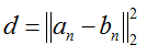
caffe_sub(
count,
bottom[0]->cpu_data(), // a
bottom[1]->cpu_data(), // b
diff_.mutable_cpu_data()); // a_i-b_i
const int channels = bottom[0]->channels();
Dtype margin = this->layer_param_.contrastive_loss_param().margin();
Dtype loss(0.0);
for (int i = 0; i < bottom[0]->num(); ++i) {
dist_sq_.mutable_cpu_data()[i] = caffe_cpu_dot(channels,
diff_.cpu_data() + (i*channels), diff_.cpu_data() + (i*channels));
if (static_cast<int>(bottom[2]->cpu_data()[i])) { // similar pairs
loss += dist_sq_.cpu_data()[i];
} else { // dissimilar pairs
loss += std::max(margin-dist_sq_.cpu_data()[i], Dtype(0.0));
}
}
loss = loss / static_cast<Dtype>(bottom[0]->num()) / Dtype(2);
(*top)[0]->mutable_cpu_data()[0] = loss;
}前馈的过程很简单,按照公式进行计算就好了。另外从代码中还可以看到,在前馈的公式中y表示是否相似,是一个0,1变量。
反馈:
template <typename Dtype>
void ContrastiveLossLayer<Dtype>::Backward_cpu(const vector<Blob<Dtype>*>& top,
    const vector<bool>& propagate_down, vector<Blob<Dtype>*>* bottom) {
  Dtype margin = this->layer_param_.contrastive_loss_param().margin();
  for (int i = 0; i < 2; ++i) {
    if (propagate_down[i]) {
      const Dtype sign = (i == 0) ? 1 : -1;
      const Dtype alpha = sign * top[0]->cpu_diff()[0] /
          static_cast<Dtype>((*bottom)[i]->num());
      int num = (*bottom)[i]->num();
      int channels = (*bottom)[i]->channels();
      for (int j = 0; j < num; ++j) {
        Dtype* bout = (*bottom)[i]->mutable_cpu_diff();
        if (static_cast<int>((*bottom)[2]->cpu_data()[j])) {  // similar pairs
          caffe_cpu_axpby(
              channels,
              alpha,
              diff_.cpu_data() + (j*channels),
              Dtype(0.0),
              bout + (j*channels));
        } else {  // dissimilar pairs
          if ((margin-dist_sq_.cpu_data()[j]) > Dtype(0.0)) {
            caffe_cpu_axpby(
                channels,
                -alpha,
                diff_.cpu_data() + (j*channels),
                Dtype(0.0),
                bout + (j*channels));
          } else {
            caffe_set(channels, Dtype(0), bout + (j*channels));
          }
        }
      }
    }
  }
}
这里的计算过程也很简单,按照前面原理介绍中提到的公式来计算就好了。不过 有一个疑问,没有弄懂:
应该来说,这个层是整个网络中最后一层了,那么误差也就是在这里面计算的,也就是loss嘛,但是前馈的时候,将loss存入top.cpu_data中的。而反馈的时候,误差传递用的却是top.cpu_dff,那么top.cpu_diff是哪里来的呢?
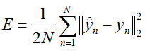
4 EuclideanLossLayer:
@brief Computes the Euclidean (L2) loss:
for real-valued regression tasks.
@param bottom input Blob vector (length 2)-# @f$ (N \times C \times H \times W) @f$
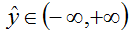
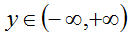
the predictions:
-# @f$ (N \times C \times H \times W) @f$
the targets
This can be used for least-squares regression tasks. An InnerProductLayer input to a EuclideanLossLayer exactly formulates a linear least squares regression problem. With non-zero weight decay the problem becomes one of ridge regression -- see src/caffe/test/test_sgd_solver.cpp for a concrete example wherein we check that the gradients computed for a Net with exactly this structure match hand-computed gradient formulas for ridge regression.
(Note: Caffe, and SGD in general, is certainly \b not the best way to solve linear least squares problems! We use it only as an instructive example.)
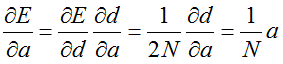
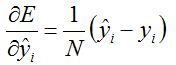
4.1 原理介绍:
前馈的过程就直接按照上面的公式计算即可;反馈的过程其实更简单,因为上面的导数:
4.2 前馈反馈函数:
template <typename Dtype>
void EuclideanLossLayer<Dtype>::Forward_cpu(const vector<Blob<Dtype>*>& bottom,
    vector<Blob<Dtype>*>* top) {
  int count = bottom[0]->count();
  caffe_sub(
      count,
      bottom[0]->cpu_data(),
      bottom[1]->cpu_data(),
      diff_.mutable_cpu_data());
  Dtype dot = caffe_cpu_dot(count, diff_.cpu_data(), diff_.cpu_data());
  Dtype loss = dot / bottom[0]->num() / Dtype(2);
  (*top)[0]->mutable_cpu_data()[0] = loss;
}

template <typename Dtype>
void EuclideanLossLayer<Dtype>::Backward_cpu(const vector<Blob<Dtype>*>& top,
    const vector<bool>& propagate_down, vector<Blob<Dtype>*>* bottom) {
  for (int i = 0; i < 2; ++i) {
    if (propagate_down[i]) {
      const Dtype sign = (i == 0) ? 1 : -1;
      const Dtype alpha = sign * top[0]->cpu_diff()[0] / (*bottom)[i]->num();
      caffe_cpu_axpby(
          (*bottom)[i]->count(),              // count
          alpha,                              // alpha
          diff_.cpu_data(),                   // a
          Dtype(0),                           // beta
          (*bottom)[i]->mutable_cpu_diff());  // b
    }
  }
}
因为这里比较简单,就不啰嗦了,只是比较奇怪的是, 为什么反馈的时候会对标签y做偏导计算呢?好奇怪!!当然如果不要将y理解成标签,将这种欧氏loss理解层和上面介绍的loss同样的效果,那么对y求偏导也是可以理解的。
5 HingeLossLayer:
@brief Computes the hinge loss for a one-of-many classification task.
@param bottom input Blob vector (length 2)
-# @f$ (N \times C \times H \times W) @f$
the predictions @f$ t @f$, a Blob with values in

indicating the predicted score for each of the
classes. In an SVM, @f$ t @f$ is the result of taking the inner product

of the D-dimensional features
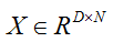
and the learned hyperplane parameters

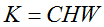
so a Net with just an InnerProductLayer (with num_output = D) providing predictions to a HingeLossLayer and no other learnable parameters or losses is equivalent to an SVM.
-# @f$ (N \times 1 \times 1 \times 1) @f$
the labels @f$ l @f$, an integer-valued Blob with values
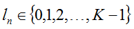
indicating the correct class label among the @f$ K @f$ classes
@param top output Blob vector (length 1)
-# @f$ (1 \times 1 \times 1 \times 1) @f$
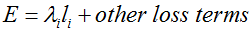
the computed hinge loss:
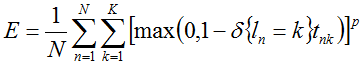
for the @f$ L^p @f$ norm
(defaults to @f$ p = 1 @f$, the L1 norm; L2 norm, as in L2-SVM, is also available), and

In an SVM,
is the result of taking the inner product
of the features

and the learned hyperplane parameters
So, a Net with just an InnerProductLayer (with num_output = @f$k@f$) providing predictions to a HingeLossLayer is equivalent to an SVM (assuming it has no other learned outside the InnerProductLayer and no other losses outside the HingeLossLayer).
5.1 原理介绍:
前馈的原理已经在上面说明了。
那么反馈的时候是怎么做的呢?
Gradients cannot be computed with respect to the label inputs (bottom[1]), so this method ignores bottom[1] and requires !propagate_down[1], crashing if propagate_down[1] is set.
@param top output Blob vector (length 1), providing the error gradient with respect to the outputs
-# @f$ (1 \times 1 \times 1 \times 1) @f$
This Blob's diff will simply contain the
as 

hence

(*Assuming that this top Blob is not used as a bottom (input) by any other layer of the Net.)
@param propagate_down see Layer::Backward.
propagate_down[1] must be false as we can't compute gradients with respect to the labels.
@param bottom input Blob vector (length 2)
-# @f$ (N \times C \times H \times W) @f$
the predictions @f$t@f$; Backward computes diff
-# @f$ (N \times 1 \times 1 \times 1) @f$
the labels -- ignored as we can't compute their error gradients

5.2 前馈和反馈函数:
前馈:
template <typename Dtype>
void HingeLossLayer<Dtype>::Forward_cpu(const vector<Blob<Dtype>*>& bottom,
    vector<Blob<Dtype>*>* top) {
  const Dtype* bottom_data = bottom[0]->cpu_data();
  Dtype* bottom_diff = bottom[0]->mutable_cpu_diff();
  const Dtype* label = bottom[1]->cpu_data();
  int num = bottom[0]->num();
  int count = bottom[0]->count();
  int dim = count / num;

  caffe_copy(count, bottom_data, bottom_diff);
  for (int i = 0; i < num; ++i) {
    bottom_diff[i * dim + static_cast<int>(label[i])] *= -1;
  }
  for (int i = 0; i < num; ++i) {
    for (int j = 0; j < dim; ++j) {
      bottom_diff[i * dim + j] = std::max(
        Dtype(0), 1 + bottom_diff[i * dim + j]);
    }
  }
  Dtype* loss = (*top)[0]->mutable_cpu_data();
  switch (this->layer_param_.hinge_loss_param().norm()) {
  case HingeLossParameter_Norm_L1:
    loss[0] = caffe_cpu_asum(count, bottom_diff) / num;
    break;
  case HingeLossParameter_Norm_L2:
    loss[0] = caffe_cpu_dot(count, bottom_diff, bottom_diff) / num;
    break;
  default:
    LOG(FATAL) << "Unknown Norm";
  }
}
这里,其实不是很难理解。从上面的计算过程来看,相当于是先将bottom_data拷贝到bottom_diff中,然后对bottom_diff中的数据一部分乘以了-1,注意,乘以-1的只是该图片对应的标签位置(可以参考手写数字识别的时候,那个标签是怎么做的)。后面开始做+1的操作,按照公式来看,其实是max(0, 1-bottom_diff),但由于bottom_diff中只是很小的一部分数据乘以了-1,所以在代码中在做+1操作时,其实对应的公式应该是

那么在前馈的公式中 t 也就是bottom_data(拷贝到了bottom_diff中)。
前馈的最后就没什么好说的,做1阶范数或者2阶范数。
反馈:
template <typename Dtype>
void HingeLossLayer<Dtype>::Backward_cpu(const vector<Blob<Dtype>*>& top,
    const vector<bool>& propagate_down, vector<Blob<Dtype>*>* bottom) {
  if (propagate_down[1]) {
    LOG(FATAL) << this->type_name()
               << " Layer cannot backpropagate to label inputs.";
  }
  if (propagate_down[0]) {
    Dtype* bottom_diff = (*bottom)[0]->mutable_cpu_diff();
    const Dtype* label = (*bottom)[1]->cpu_data();
    int num = (*bottom)[0]->num();
    int count = (*bottom)[0]->count();
    int dim = count / num;

    for (int i = 0; i < num; ++i) {
      bottom_diff[i * dim + static_cast<int>(label[i])] *= -1;
    }

    const Dtype loss_weight = top[0]->cpu_diff()[0];
    switch (this->layer_param_.hinge_loss_param().norm()) {
    case HingeLossParameter_Norm_L1:
      caffe_cpu_sign(count, bottom_diff, bottom_diff);
      caffe_scal(count, loss_weight / num, bottom_diff);
      break;
    case HingeLossParameter_Norm_L2:
      caffe_scal(count, loss_weight * 2 / num, bottom_diff);
      break;
    default:
      LOG(FATAL) << "Unknown Norm";
    }
  }
}
前馈中的max(0, 1 - {l_n = k} t_nk)令为f,那么对t_nk的偏导可以写为:(2-范数为例)
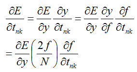
在别的地方看到:
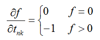
其实不太理解这是为什么!!!因为 f>0 的地方为啥只能是 l_n=k 的时候呢?
6 InfogainLossLayer:
A generalization of MultinomialLogisticLossLayer that takes an "information gain" (infogain) matrix specifying the "value" of all label pairs.
6.1 原理介绍:
输入:
-
形状:


 预测值
预测值


 内, 表示这预测每一类的概率,共

 个类, 每一个预测 概率
 的和为1:
的和为1:


 .
. -
形状:
标签值:
 , 是一个整数值,其范围是


 表示着在
个类中的索引。
表示着在
个类中的索引。 -
形状:
(可选) 信息增益矩阵
.作为第三个输入参数,. 如果
 , 则它等价于多项式逻辑损失函数
输出:
形状:
计算公式:


 , 其中
表示 行
of
.
, 其中
表示 行
of
.
6.2 属性变量:
Blob<Dtype> infogain_;这个变量也就是前面介绍的H。
6.3 构造函数:
template <typename Dtype>
void InfogainLossLayer<Dtype>::LayerSetUp(
    const vector<Blob<Dtype>*>& bottom, vector<Blob<Dtype>*>* top) {
  LossLayer<Dtype>::LayerSetUp(bottom, top);
  if (bottom.size() < 3) {
    CHECK(this->layer_param_.infogain_loss_param().has_source())
        << "Infogain matrix source must be specified.";
    BlobProto blob_proto;
    ReadProtoFromBinaryFile(
      this->layer_param_.infogain_loss_param().source(), &blob_proto);
    infogain_.FromProto(blob_proto);
  }
}

template <typename Dtype>
void InfogainLossLayer<Dtype>::Reshape(
    const vector<Blob<Dtype>*>& bottom, vector<Blob<Dtype>*>* top) {
  LossLayer<Dtype>::Reshape(bottom, top);
  Blob<Dtype>* infogain = NULL;
  if (bottom.size() < 3) {
    infogain = &infogain_;
  } else {
    infogain = bottom[2];
  }
  CHECK_EQ(bottom[1]->channels(), 1);
  CHECK_EQ(bottom[1]->height(), 1);
  CHECK_EQ(bottom[1]->width(), 1);
  const int num = bottom[0]->num();
  const int dim = bottom[0]->count() / num;
  CHECK_EQ(infogain->num(), 1);
  CHECK_EQ(infogain->channels(), 1);
  CHECK_EQ(infogain->height(), dim);
  CHECK_EQ(infogain->width(), dim);
}
从这里可以看到,当输入的bottom只有两个时,H矩阵是需要被指定的。如果输入bottom有三个时,第三个bottom就作为H矩阵。
6.4 前馈和反馈函数:
前馈:
template <typename Dtype>
void InfogainLossLayer<Dtype>::Forward_cpu(const vector<Blob<Dtype>*>& bottom,
    vector<Blob<Dtype>*>* top) {
  const Dtype* bottom_data = bottom[0]->cpu_data();
  const Dtype* bottom_label = bottom[1]->cpu_data();
  const Dtype* infogain_mat = NULL;
  if (bottom.size() < 3) {
    infogain_mat = infogain_.cpu_data();
  } else {
    infogain_mat = bottom[2]->cpu_data();
  }
  int num = bottom[0]->num();
  int dim = bottom[0]->count() / bottom[0]->num();
  Dtype loss = 0;
  for (int i = 0; i < num; ++i) {
    int label = static_cast<int>(bottom_label[i]);
    for (int j = 0; j < dim; ++j) {
      Dtype prob = std::max(bottom_data[i * dim + j], Dtype(kLOG_THRESHOLD));
      loss -= infogain_mat[label * dim + j] * log(prob);
    }
  }
  (*top)[0]->mutable_cpu_data()[0] = loss / num;
}
反馈:
template <typename Dtype>
void InfogainLossLayer<Dtype>::Backward_cpu(const vector<Blob<Dtype>*>& top,
    const vector<bool>& propagate_down,
    vector<Blob<Dtype>*>* bottom) {
  if (propagate_down[1]) {
    LOG(FATAL) << this->type_name()
               << " Layer cannot backpropagate to label inputs.";
  }
  if (propagate_down.size() > 2 && propagate_down[2]) {
    LOG(FATAL) << this->type_name()
               << " Layer cannot backpropagate to infogain inputs.";
  }
  if (propagate_down[0]) {
    const Dtype* bottom_data = (*bottom)[0]->cpu_data();
    const Dtype* bottom_label = (*bottom)[1]->cpu_data();
    const Dtype* infogain_mat = NULL;
    if (bottom->size() < 3) {
      infogain_mat = infogain_.cpu_data();
    } else {
      infogain_mat = (*bottom)[2]->cpu_data();
    }
    Dtype* bottom_diff = (*bottom)[0]->mutable_cpu_diff();
    int num = (*bottom)[0]->num();
    int dim = (*bottom)[0]->count() / (*bottom)[0]->num();
    const Dtype scale = - top[0]->cpu_diff()[0] / num;
    for (int i = 0; i < num; ++i) {
      const int label = static_cast<int>(bottom_label[i]);
      for (int j = 0; j < dim; ++j) {
        Dtype prob = std::max(bottom_data[i * dim + j], Dtype(kLOG_THRESHOLD));
        bottom_diff[i * dim + j] = scale * infogain_mat[label * dim + j] / prob;
      }
    }
  }
}


 804
804


 被折叠的 条评论
为什么被折叠?
被折叠的 条评论
为什么被折叠?
 到【灌水乐园】发言


