pytorch实现GRU（附code）

接上一篇文章（pytorch实现LSTM），在实现LSTM之后，又发现了GRU网络。

说GRU是LSTM网络的一种效果很好的变体，它较LSTM网络的结构更加简单，而且效果也很好，也是当前非常流形的一种网络。

所以决定尝试一下！

注：数据集仍然使用上文中的IGBT加速老化数据集(3)，数据与处理方法不变，直接上代码！！！

在保证输入样本参数和学习率不变的情况下，即input_size = 5，out_oput = 1，lr = 0.01，试了很多参数，发现在训练集80%，测试集20%，hidden_size = 30，使用两个全连接层时结果最好，与上文的LSTM效果接近（代码为CPU版本哦）。

（说好的更简单，效果更好，不明白为啥使用的隐藏层和全连接层要更多了？？？）

import scipy.io as sio
import numpy as np
import torch
from torch import nn
import matplotlib.pyplot as plt
import matplotlib
import pandas as pd
from torch.autograd import Variable
import math
import csv

# Define LSTM Neural Networks
class GruRNN(nn.Module):
    """
        Parameters：
        - input_size: feature size
        - hidden_size: number of hidden units
        - output_size: number of output
        - num_layers: layers of LSTM to stack
    """

    def __init__(self, input_size, hidden_size=1, output_size=1, num_layers=1):
        super().__init__()

        self.gru = nn.GRU(input_size, hidden_size, num_layers)  # utilize the GRU model in torch.nn
        self.linear1 = nn.Linear(hidden_size, 16) # 全连接层
        self.linear2 = nn.Linear(16, output_size) # 全连接层

    def forward(self, _x):
        x, _ = self.gru(_x)  # _x is input, size (seq_len, batch, input_size)
        s, b, h = x.shape  # x is output, size (seq_len, batch, hidden_size)
        x = x.view(s * b, h)
        x = self.linear1(x)
        x = self.linear2(x)
        x = x.view(s, b, -1)
        return x

if __name__ == '__main__':

    # checking if GPU is available
    device = torch.device("cpu")

    if (torch.cuda.is_available()):
        device = torch.device("cuda:0")
        print('Training on GPU.')
    else:
        print('No GPU available, training on CPU.')

    # 数据读取&类型转换
    data_x = np.array(pd.read_csv('Data_x.csv', header=None)).astype('float32')
    data_y = np.array(pd.read_csv('Data_y.csv', header=None)).astype('float32')

    # 数据集分割
    data_len = len(data_x)
    t = np.linspace(0, data_len, data_len + 1)

    train_data_ratio = 0.8  # Choose 80% of the data for training
    train_data_len = int(data_len * train_data_ratio)

    train_x = data_x[5:train_data_len]
    train_y = data_y[5:train_data_len]
    t_for_training = t[5:train_data_len]

    test_x = data_x[train_data_len:]
    test_y = data_y[train_data_len:]
    t_for_testing = t[train_data_len:]

    # ----------------- train -------------------
    train_x_tensor = train_x.reshape(5, -1, 1)
    train_y_tensor = train_y.reshape(1, -1, 1)

    # transfer data to pytorch tensor
    train_x_tensor = torch.from_numpy(train_x_tensor)
    train_y_tensor = torch.from_numpy(train_y_tensor)

    gru_model = GruRNN(1, 30, output_size=1, num_layers=1)  # 30 hidden units
    print('GRU model:', gru_model )
    print('model.parameters:', gru_model .parameters)
    print('train x tensor dimension:', Variable(train_x_tensor).size())

    criterion = nn.MSELoss()
    optimizer = torch.optim.Adam(gru_model .parameters(), lr=1e-2)

    prev_loss = 1000
    max_epochs = 3000

    train_x_tensor = train_x_tensor.to(device)

    for epoch in range(max_epochs):
        output = gru_model(train_x_tensor).to(device)
        loss = criterion(output, train_y_tensor)

        optimizer.zero_grad()
        loss.backward()
        optimizer.step()

        if loss < prev_loss:
            torch.save(gru_model.state_dict(), 'lstm_model.pt')  # save model parameters to files
            prev_loss = loss

        if loss.item() < 1e-4:
            print('Epoch [{}/{}], Loss: {:.5f}'.format(epoch + 1, max_epochs, loss.item()))
            print("The loss value is reached")
            break
        elif (epoch + 1) % 100 == 0:
            print('Epoch: [{}/{}], Loss:{:.5f}'.format(epoch + 1, max_epochs, loss.item()))

    # prediction on training dataset
    pred_y_for_train = gru_model(train_x_tensor).to(device)
    pred_y_for_train = pred_y_for_train.view(-1, OUTPUT_FEATURES_NUM).data.numpy()

    # ----------------- test -------------------
    gru_model = gru_model .eval()  # switch to testing model

    # prediction on test dataset
    test_x_tensor = test_x.reshape(1, -1, 5)
    test_x_tensor = torch.from_numpy(test_x_tensor)  # 变为tensor
    test_x_tensor = test_x_tensor.to(device)

    pred_y_for_test = gru_model(test_x_tensor).to(device)
    pred_y_for_test = pred_y_for_test.view(-1, OUTPUT_FEATURES_NUM).data.numpy()

    loss = criterion(torch.from_numpy(pred_y_for_test), torch.from_numpy(test_y))
    print("test loss：", loss.item())

    # ----------------- plot -------------------
    plt.figure()
    plt.plot(t_for_training, train_y, 'b', label='y_trn')
    plt.plot(t_for_training, pred_y_for_train, 'y--', label='pre_trn')

    plt.plot(t_for_testing, test_y, 'k', label='y_tst')
    plt.plot(t_for_testing, pred_y_for_test, 'm--', label='pre_tst')

    plt.xlabel('t')
    plt.ylabel('Vce')
    plt.show()

结果如下图所示：

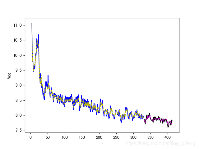
蓝线代表训练集真实值，黄线代表训练集预测值

黑线代表测试集真实值，紫线代表测试集预测值

test_loss=0.0038289446383714676

上篇文章有数据集和代码哦。