数学体操之牛顿数值法解方程的程序和图解

papaofdoudou

已于 2023-10-26 11:50:15 修改

阅读量800

点赞数 2

分类专栏：数学工程方法论文章标签： c++ 算法 c语言

于 2023-04-16 13:59:49 首次发布

本文链接：https://blog.csdn.net/tugouxp/article/details/130181394

版权

数学同时被 3 个专栏收录

144 篇文章 19 订阅

订阅专栏

工程

52 篇文章 1 订阅

订阅专栏

方法论

7 篇文章 1 订阅

订阅专栏

牛顿法是一种用来寻找函数零点的迭代方法，它基于以下思路，如果我们知道了一个函数在某个点的切线，那么函数的零点就可以通过切线与x轴的交点来近似计算。

给定一个函数 $f(x)$ ,找到零点 $x_0$ ,过程如下:

选择初始点 $x_1$ ,然后使用这个点处的切线来近似 $f(x)$ ,也就是说，找到下面这条直线与x轴的家的交点x1,

$y-f(x_0)=f'(x_0)(x-x_0)$

$0 -f(x_0)=f'(x_0)(x_1-x_0)\Rightarrow x_1 =x_0 - \frac{f(x_0)}{f`(x_0)}$

这样，我们可以通过将其与x轴相交一获得更接近真实零点的新估计值 $x_2$ :

$0-f(x_1)=f'(x_1)(x-x_1)\Rightarrow x_2 =x_1 -\frac{f(x_1)}{f'(x_1)}$

所以，得到了递推公式为：

$x_{n+1}=x_n- \frac{f(x_n)}{f'(x_n)}$

从上式可以看出，如果我们对 $x_1$ 一次，则可以计算出一个更好的估计值 $x_2$ ,然后我们可以不断重复此过程，直到达到我们满意的精度或次数为止。

下面举例说明：

用牛顿法求解一元二次方程，程序比较简单，利用导函数与横轴的交点的横坐标不断迭代即可，程序清单如下：

#include <stdio.h>
#include <stdlib.h>
#include <math.h>

//newton methond to get the root of
//equation of two degree f(x) = x^2-8x+9
//the deritive is f'(x) = 2x - 8;
static void newton_methed(void)
{
	// init value of start point. 
	double x1 = 8.0, x2=0.0, y1, root;
	double k; // the gradient of f(x)

	while(fabs(x1-x2) > 1e-6) {
		x2=x1;

		k = 2 * x1 - 8;
		y1 = x1*x1 - 8*x1 + 9;

		root = (-1 * y1)/k + x1;  //according y-y1=k(x-x1)
		x1 = root;

		printf("root is %f.\n", root);
	}

	return;
}

int main(void)
{
	newton_methed();

	return 0;
}

图解说明：

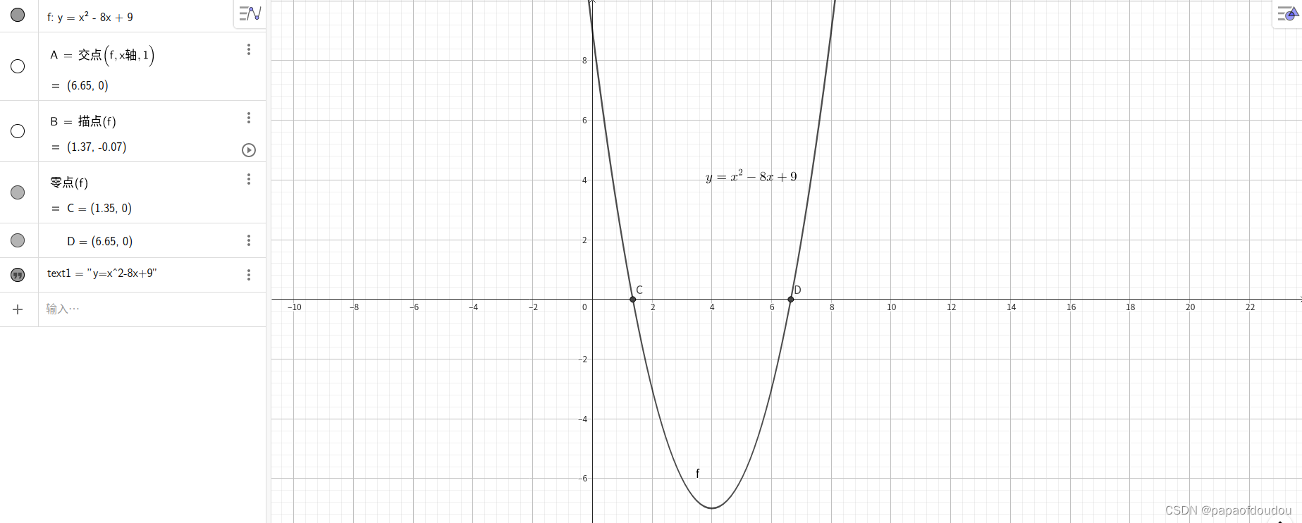
下图展示了迭代过程：

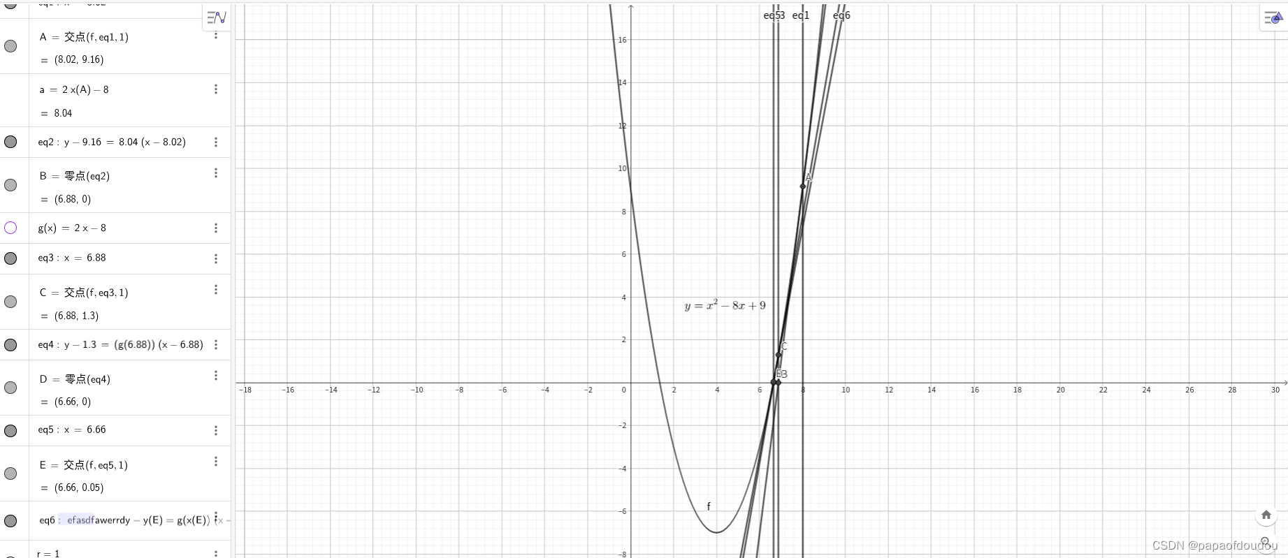
根值到了极度接近的阶段，宏观上已经看不出切线和坐标轴的交点，即便放大绘图，也会感受到工具渲染非常的吃力。下图展示了三次迭代后的效果，左边是原函数和坐标轴的交点，邮编是三伦迭代的切线和X轴的交点，可以看到，交点非常的接近了。

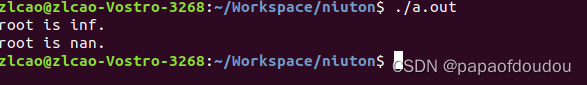
如果将迭代初始值甚至为一元二次函数的极点位置，程序将失效，原因是此时极点的切线位置和X轴平行，没有交点，算法无法执行下去。

对于这个例子来说，如果将初始的X1设置为4，算法将会输出非法值。

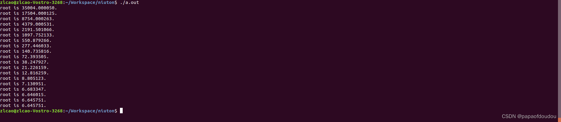
但是只要打破平衡，稍微偏离极点中心哪怕一点点，算法将给出正确的值，如果向左偏离，则得到左交点，如果向右偏离，将得到右交点，结合图形，很容易理解这些结论。

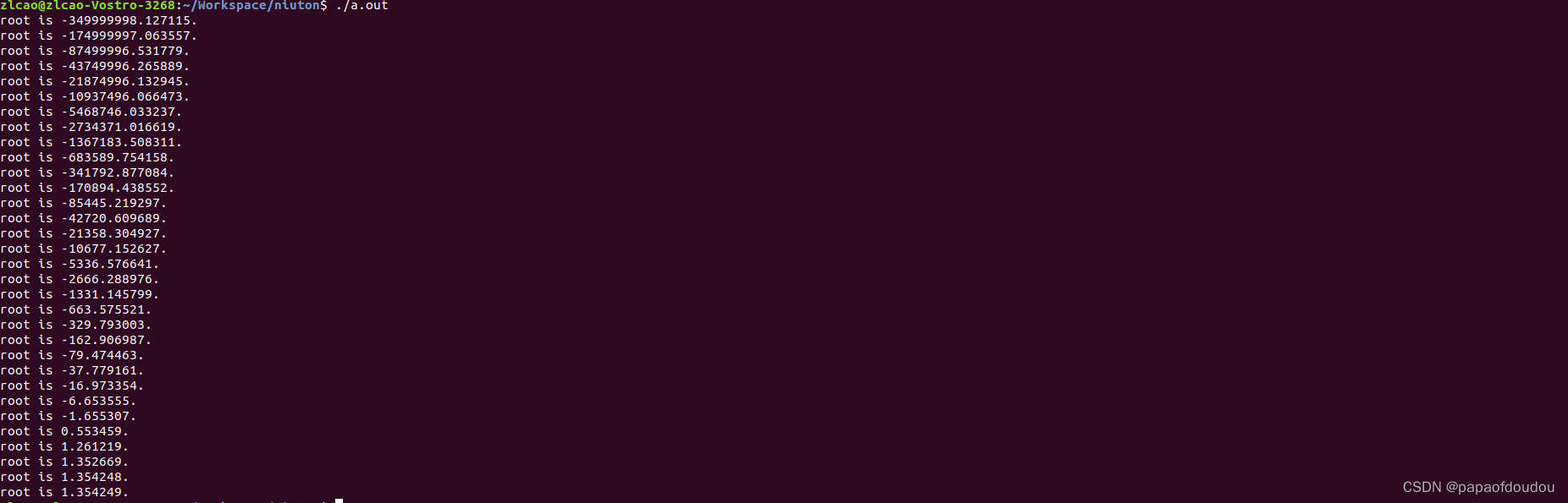
计算左边根的迭代示意图

一个不算简单的解方程问题，数形结合起来后，直观了很多，看来数学从高的观点往下看，往往会更有收获。

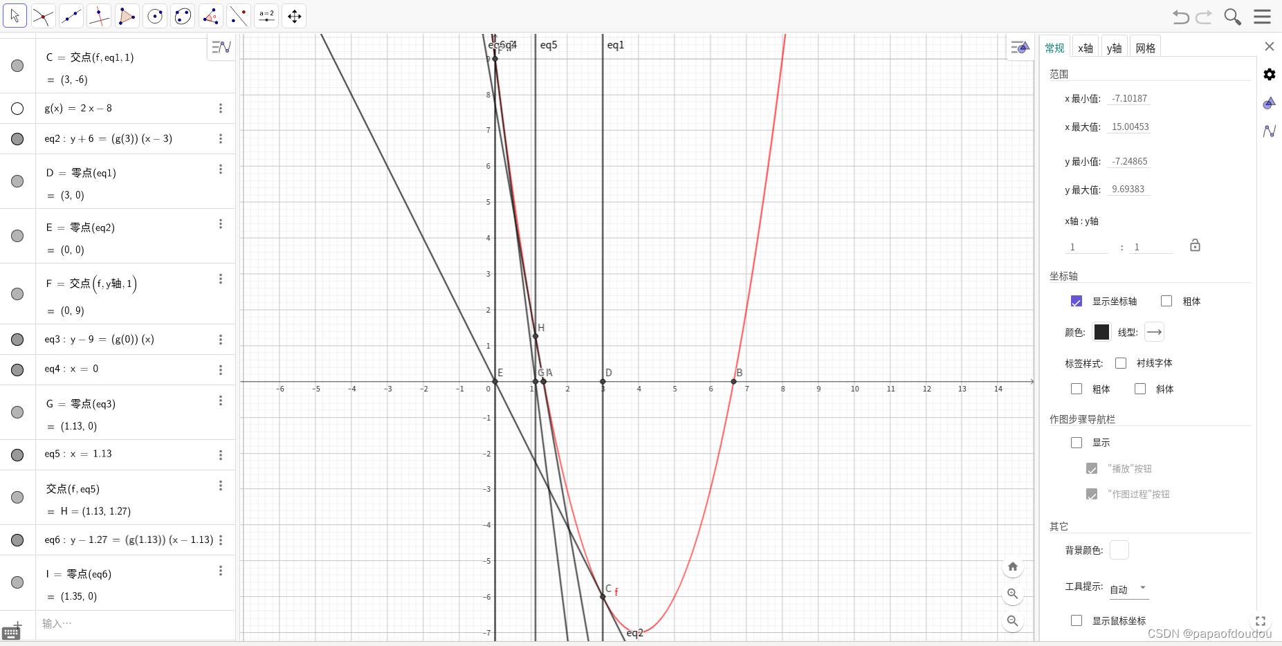
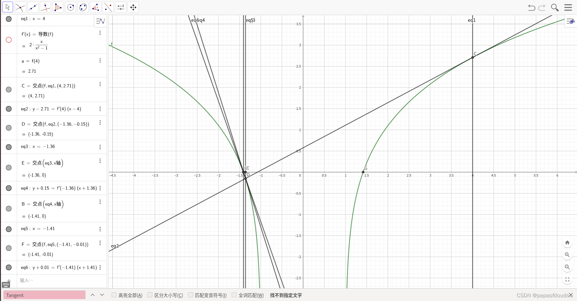
一个新的例子，自然对数求根：

geogebra得到的两个根是+/- 1.41.

程序：

#include <stdio.h>
#include <stdlib.h>
#include <math.h>

//newton methond to get the root of
//equation of two degree f(x) = x^2-8x+9
//the deritive is f'(x) = 2x - 8;
static void newton_methed1(void)
{
	// init value of start point. 
	double x1 = 3.99999999, x2=0.0, y1, root;
	double k; // the gradient of f(x)

	while(fabs(x1-x2) > 1e-6) {
		x2=x1;

		k = 2 * x1 - 8;
		y1 = x1*x1 - 8*x1 + 9;

		root = (-1 * y1)/k + x1;  //according y-y1=k(x-x1)
		x1 = root;

		printf("root is %f.\n", root);
	}

	return;
}

//newton methond to get the root of
//equation of two degree f(x) = log(x^2-1)
//the deritive is f'(x) = 2x/(x^2-1);
static void newton_methed2(float x1)
{
	// init value of start point. 
	double x2=0.0, y1, root;
	double k; // the gradient of f(x)

	while(fabs(x1-x2) > 1e-6) {
		x2=x1;

		k = 2 * x1/(x1*x1 - 1);
		y1 = log(x1*x1-1);

		root = (-1 * y1)/k + x1;  //according y-y1=k(x-x1)
		x1 = root;

		printf("root is %f.\n", root);
	}

	return;
}

int main(void)
{
	//newton_methed1();
	newton_methed2(3.999999999);
	newton_methed2(-3.999999999);

	return 0;
}

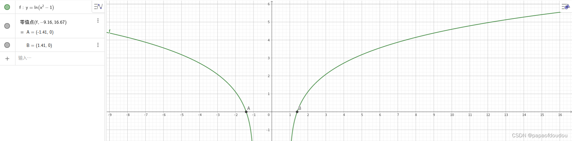
程序迭代过程，最终得到了正确的根：

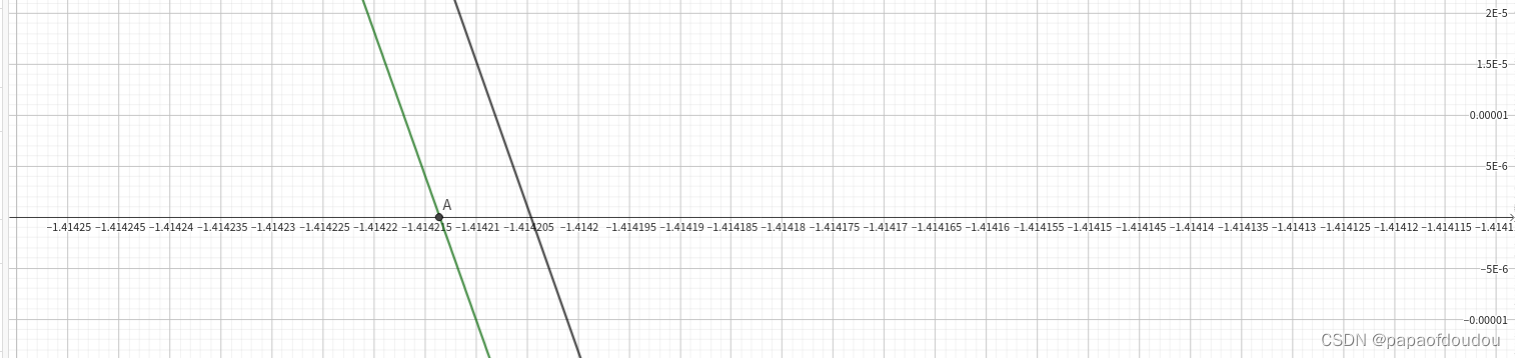
迭代数次后的逼近位置：

这个例子中实际上触发了牛顿法的一个limitation,叫做root jumping,它描述了这样一种缺陷，当函数有多个根，你选择距离某个根比较近的值作为初始值，试图通过牛顿法得到这个根的时候，你实际得到的可能是另外的根。就拿上面的例子来说，初始值3.999999距离正根比较近，但是牛顿法得到的却是-1.4142.选择负值做初始值时恰好相反，如下图所示：

程序失效的情况

在局部极值附近的情况下，算法会进入振荡周期，程序进入错误的死循环状态：

#include <stdio.h>
#include <stdlib.h>
#include <math.h>

//newton methond to get the root of
//equation of two degree f(x) = x^2 + 1
//the deritive is f'(x) = 2x;
static void newton_methed1(void)
{
	// init value of start point. 
	double x1 = 3.99999999, x2=0.0, y1, root;
	double k; // the gradient of f(x)

	while(fabs(x1-x2) > 1e-6) {
		x2=x1;

		k = 2 * x1;
		y1 = x1*x1 + 1;

		root = (-1 * y1)/k + x1;  //according y-y1=k(x-x1)
		x1 = root;

		printf("root is %f.\n", root);
	}

	return;
}

//newton methond to get the root of
//equation of two degree f(x) = log(x^2-1)
//the deritive is f'(x) = 2x/(x^2-1);
static void newton_methed2(float x1)
{
	// init value of start point. 
	double x2=0.0, y1, root;
	double k; // the gradient of f(x)

	while(fabs(x1-x2) > 1e-6) {
		x2=x1;

		k = 2 * x1/(x1*x1 - 1);
		y1 = log(x1*x1-1);

		root = (-1 * y1)/k + x1;  //according y-y1=k(x-x1)
		x1 = root;

		printf("root is %f.\n", root);
	}

	return;
}

int main(void)
{
	newton_methed1();
	//newton_methed2(3.999999999);
	//newton_methed2(-3.999999999);

	return 0;
}

一幅图演示算法过程:

下面是卡马克大神优化过的牛顿法实现，只要一步迭代，就可以获得满足精度要求的根，核心思想是寻找一个接近根的初始值开始迭代，这个优化依赖于IEEE7554浮点数格式的二进制定义，感兴趣可以网上搜索一下优化思路。

从著名的q_rsqrt说起 - 知乎

#include <stdio.h>
#include <stdlib.h>
#include <math.h>

float rsqrt(float number) //这是卡马克大神级别的优化
{
    long i;
    float x2, y;
    const float threehalfs = 1.5F;
   
    x2 = number * 0.5F;
    y  = number;
    i  = * ( long * ) &y;      // evil floating point bit level hacking
    i  = 0x5f3759df - ( i >> 1 );               // what the fuck?
    y  = * ( float * ) &i;
    y  = y * ( threehalfs - ( x2 * y * y ) );   // 1st iteration

    return y;
}

int main(void)
{
    printf("%s line %d, %f, %f.\n", __func__, __LINE__, rsqrt(2.0), 1.0/sqrt(2.0));

    return 0;
}

总结：

牛顿法的主要优点是，它在每次迭代中都收敛在的非常快，在实践中被证明比其他迭代方法更快，但是它也有缺点:

1,就像例子中看到的，当函数具有多个局部零点时，算法的初始值可能导致收敛到错误的根。

2.算法需要有解析式表达的导数计算方法。

3.可能会发生根跳转，得不到预期的结果。

4.在局部极值附近可能会发生振荡导致收敛变慢，无法跳脱。

5.拐点可能导致算法实效。

解方程是一种近似数学，虽然有的时候能够获得方程的解析式，但大多数的时候（5次及以上的普通方程）是没有解析式的，这个时候只能通过数值解法得到近似解。即便对于有解析式可解方程，通常根也是无理数，没有精确解，所以解方程实际上是一件“差不多”就可以的事，所以计算机能够很好的胜任这份工作。

结束

papaofdoudou

关注

2
点赞
踩
0

收藏

觉得还不错? 一键收藏
打赏
0
评论
数学体操之牛顿数值法解方程的程序和图解

牛顿法的主要优点是，它在每次迭代中都收敛在的非常快，在实践中被证明比其他迭代方法更快，但是它也有缺点:1,就像例子中看到的，当函数具有多个局部零点时，算法的初始值可能导致收敛到错误的根。2.算法需要有解析式表达的导数计算方法。3.可能会发生根跳转，得不到预期的结果。4.在局部极值附近可能会发生振荡导致收敛变慢，无法跳脱。5.拐点可能导致算法实效。解方程是一种近似数学，虽然有的时候能够获得方程的解析式，但大多数的时候（5次及以上的普通方程）是没有解析式的，这个时候只能通过数值解法得到近似解。
复制链接

扫一扫