


 本文深入探讨了使用矩阵运算解决图算法的问题,包括连通分支的定义、传统算法实现、基于矩阵的实现方法及其优缺点。文章还提供了Python代码实现,并详细解释了算法背后的理论基础。
1.连通分支
连通分支(Connected Component)是指:在一个图中,某个子图的任意两点有边连接,并且该子图去剩下的任何点都没有边相连。在 Wikipedia上的定义如下:In graph theory, a connected component (or just component) of an undirected graph is a subgraph in which any two vertices are connected to each other by paths, and which is connected to no additional vertices in the supergraph.
如Wikipedia上给的例子:
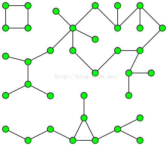
根据定义不难看出该图有三个连通分支。
另外,连通分支又分为弱连通分支和强连通分支。强连通分支是指子图点i可以连接到点j,同时点j也可以连接到点i。弱连通(只对有向图)分支是指子图点i可以连接到点j,但是点j可以连接不到点i。
2.传统算法
2.1算法思想
在传统算法中,我们是根据一点任意点,去找它的邻结点,然后再根据邻结点,找它的邻结点,直到所有的点遍历完。如下图: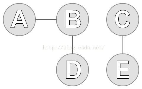
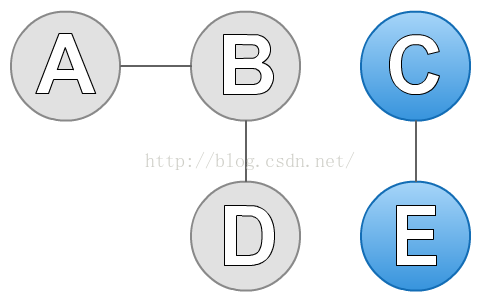
图中有A、B、C、D和E五个点。我们先任选一个点C,然后找到C的邻结点E。然后我们再找E的邻结点,发现只有C,但是我们之前遍历过C,所以排除C。现在我们没有点可以遍历了,于是找到了第一个连通分支,如下蓝色标记:
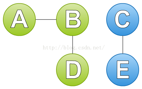
接着,我们再从没有遍历的点(A、B、C)中任选一个点A。按照上述的方法,找到A的邻结点B。然后在找B的邻结点,找到A和D,但是A我们之前遍历过,所以排除A,只剩下了D。再找D的邻结点,找到B,同样B之前也遍历过了,所以也排除B,最后发现也没有点可以访问了。于是,就找到了第二个连通分支。到此图中所有的点已经遍历完了,因此该图有两个连通分支(A、B、D)和(C、E)。如下图:
2.2算法实现
下面是用Python实现的代码:class Data(object):
def __init__(self, name):
self.__name = name
self.__links = set()
@property
def name(self):
return self.__name
@property
def links(self):
return set(self.__links)
def add_link(self, other):
self.__links.add(other)
other.__links.add(self)
# The function to look for connected components.
def connected_components(nodes):
# List of connected components found. The order is random.
result = []
# Make a copy of the set, so we can modify it.
nodes = set(nodes)
# Iterate while we still have nodes to process.
while nodes:
# Get a random node and remove it from the global set.
n = nodes.pop()
print(n)
# This set will contain the next group of nodes connected to each other.
group = {n}
# Build a queue with this node in it.
queue = [n]
# Iterate the queue.
# When it's empty, we finished visiting a group of connected nodes.
while queue:
# Consume the next item from the queue.
n = queue.pop(0)
# Fetch the neighbors.
neighbors = n.links
# Remove the neighbors we already visited.
neighbors.difference_update(group)
# Remove the remaining nodes from the global set.
nodes.difference_update(neighbors)
# Add them to the group of connected nodes.
group.update(neighbors)
# Add them to the queue, so we visit them in the next iterations.
queue.extend(neighbors)
# Add the group to the list of groups.
result.append(group)
# Return the list of groups.
return result
# The test code...
if __name__ == "__main__":
# The first group, let's make a tree.
a = Data("a")
b = Data("b")
c = Data("c")
d = Data("d")
e = Data("e")
f = Data("f")
a.add_link(b) # a
a.add_link(c) # / \
b.add_link(d) # b c
c.add_link(e) # / / \
c.add_link(f) # d e f
# The second group, let's leave a single, isolated node.
g = Data("g")
# The third group, let's make a cycle.
h = Data("h")
i = Data("i")
j = Data("j")
k = Data("k")
h.add_link(i) # h————i
i.add_link(j) # | |
j.add_link(k) # | |
k.add_link(h) # k————j
# Put all the nodes together in one big set.
nodes = {a, b, c, d, e, f, g, h, i, j, k}
# Find all the connected components.
number = 1
for components in connected_components(nodes):
names = sorted(node.name for node in components)
names = ", ".join(names)
print("Group #%i: %s" % (number, names))
number += 1
# You should now see the following output:
# Group #1: a, b, c, d, e, f
# Group #2: g
# Group #3: h, i, j, k
3.基于矩阵的实现算法
3.1理论基础
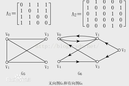
1.邻接矩阵邻接矩阵表示顶点之间相邻关系的矩阵,同时邻接矩阵分为有向邻接矩阵和无向邻接矩阵,如:
2.回路计算
假设有邻接矩阵

其中,

3.2算法推导
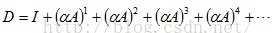
如果把经过0、1、2、3••••••条路径形成的回路矩阵求并集(注:经过0条路径形成的回路矩阵即为单位矩阵I),那么该并集C可以表示所有回路的总和,用公式可以表示为: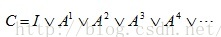
 的(i,j)有非0值,表示点i和点j是同一个强连通的集合。
由于
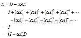
比较复杂,但是,我们可以用下式计算:
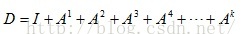
对于D,这个式子几乎不收敛,因为我们需要修改它。现在让我们考虑式子
 ,证明如下:
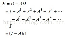
因此,

 ,使得用
,使得用
 代替A,则D重新定义为:
同理,由
可以求得:

其中,矩阵D中非0值所在列相同的行,属于同一个连通分支,即行结构相同的是一个连通分支。
3.3算法实现
下面是用Python实现的代码:from numpy.random import rand
import numpy as np
#利用求并集和交集的方法
def cccomplex(adjacencyMat):
def power(adjacencyMatPower, adjacencyMat):
adjacencyMatPower *= adjacencyMat
return adjacencyMatPower
dimension = np.shape(adjacencyMat)[0]
eye = np.mat(np.eye(dimension))
adjacencyMat = np.mat(adjacencyMat)
adjacencyMatPower = adjacencyMat.copy()
result = np.logical_or(eye, adjacencyMat)
for i in range(dimension):
adjacencyMatPower = power(adjacencyMatPower, adjacencyMat)
result = np.logical_or(result, adjacencyMatPower)
final = np.logical_and(result, result.T)
return final
#利用求矩阵逆的方法
def connectedConponents(adjacencyMat, alpha = 0.5):
n = np.shape(adjacencyMat)[0]
E = np.eye(n)
ccmatrix = np.mat(E - alpha * adjacencyMat)
return ccmatrix.I
def init(dimension):
mat = np.ones((dimension, dimension))
mat[(rand(dimension) * dimension).astype(int), (rand(dimension) * dimension).astype(int)] = 0
return mat
if __name__ == "__main__":
dimension = 4
adjacencyMat = init(dimension)
adjacencyMat1 = np.array([[0,1,0,0,0,0,0,0], [0,0,1,0,1,1,0,0],
[0,0,0,1,0,0,1,0],
[0,0,1,0,0,0,0,1],
[1,0,0,0,0,1,0,0],
[0,0,0,0,0,0,1,0],
[0,0,0,0,0,1,0,1],
[0,0,0,0,0,0,0,1]])
adjacencyMat2 = np.array([[0,1,1,0],[1,0,0,0],[1,0,0,0],[0,0,0,0]])
print(cccomplex(adjacencyMat1)) #(A, B, E) (C, D) (F, G) (H)
print(connectedConponents(adjacencyMat2))
#[[ True True False False True False False False]
# [ True True False False True False False False]
# [False False True True False False False False]
# [False False True True False False False False]
# [ True True False False True False False False]
# [False False False False False True True False]
# [False False False False False True True False]
# [False False False False False False False True]]
#[[ 2. 1. 1. 0. ]
# [ 1. 1.5 0.5 0. ]
# [ 1. 0.5 1.5 0. ]
# [ 0. 0. 0. 1. ]]
4.评价
基于矩阵运算实现的图算法,有以下几点优势:- 易于实现。利用矩阵可以仅仅通过矩阵与矩阵或矩阵与向量的运算就可以实现一些图算法。
- 易于并行。在超大矩阵运算中,可以采用分块的方式平行处理矩阵运算。同理,也可以很容易的移植分布式上(可以参考我的博文基于Spark实现的超大矩阵运算)。
- 效率更高。基于矩阵的图形算法更清晰突出的数据访问模式,可以很容易地优化(实验测试工作已完成)。
- 易于理解。这个需要对离散数学或者图论有一定基础,知道每一步矩阵运算所对应的物理意义或数学意义。


 1197
1197


 被折叠的 条评论
为什么被折叠?
被折叠的 条评论
为什么被折叠?
 到【灌水乐园】发言


