DBNet详解

最新推荐文章于 2024-05-12 11:00:00 发布

lexi_qi

最新推荐文章于 2024-05-12 11:00:00 发布

阅读量9.9k

点赞数 15

分类专栏： OCR

本文链接：https://blog.csdn.net/u010901792/article/details/112656503

版权

OCR 专栏收录该内容

2 篇文章 1 订阅

订阅专栏

创新点

本文的最大创新点。在基于分割的文本检测网络中，最终的二值化map都是使用的固定阈值来获取，并且阈值不同对性能影响较大。本文中，对每一个像素点进行自适应二值化，二值化阈值由网络学习得到，彻底将二值化这一步骤加入到网络里一起训练，这样最终的输出图对于阈值就会非常鲁棒。

和常规基于语义分割算法的区别是多了一条threshold map分支，该分支的主要目的是和分割图联合得到更接近二值化的二值图，属于辅助分支。其余操作就没啥了。整个核心知识就这些了。

算法的整体架构

首先，图像输入特征提取主干，提取特征；
其次，特征金字塔上采样到相同的尺寸，并进行特征级联得到特征F；
然后，特征F用于预测概率图（probability map P）和阈值图(threshold map T)
最后，通过P和F计算近似二值图（approximate binary map B）

在训练期间对P，T，B进行监督训练，P和B是用的相同的监督信号(label)。在推理时，只需要P或B就可以得到文本框。

网络输出：

1.probability map, wh1 , 代表像素点是文本的概率

2.threshhold map, wh1, 每个像素点的阈值

3.binary map, wh1, 由1,2计算得到，计算公式为DB公式

自适应阈值（Adaptive threshhold）

文中指出传统的文本检测算法主要是图中蓝色线，处理流程如下：

首先，通过设置一个固定阈值将分割网络训练得到的概率图(segmentation map)转化为二值图(binarization map);
然后，使用一些启发式技术(例如像素聚类)将像素分组为文本实例。

而DBNet使用红色线，思路：

通过网络去预测图片每个位置处的阈值，而不是采用一个固定的值，这样就可以很好将背景与前景分离出来，但是这样的操作会给训练带来梯度不可微的情况，对此对于二值化提出了一个叫做Differentiable Binarization来解决不可微的问题。

阈值图(threshhold map)使用流程如图2所示，使用阈值map和不使用阈值map的效果对比如图6所示，从图6©中可以看到，即使没用带监督的阈值map，阈值map也会突出显示文本边界区域，这说明边界型阈值map对最终结果是有利的。所以，本文在阈值map上选择监督训练，已达到更好的表现

二值化

标准二值化

一般使用分割网络（segmentation network）产生的概率图（probability map P），将P转化为一个二值图P，当像素为1的时候，认定其为有效的文本区域，同时二值处理过程：

i和j代表了坐标点的坐标，t是预定义的阈值；

可微二值(differentiable Binarization)

公式1是不可微的，所以没法直接用于训练，本文提出可微的二值化函数，如下（其实就是一个带系数的sigmoid）：

就是近似二值图；T代表从网络中学习到的自适应阈值图；k是膨胀因子（经验性设置k=50）.

这个近似的二值化函数的表现类似于标准的二值化函数，如图4所表示，但是因为可微，所以可以直接用于网络训练，基于自适应阈值可微二值化不仅可以帮助区分文本区域和背景，而且可以将连接紧密的文本实例分离出来。

为了说明DB模块的引入对于联合训练的优势，作者对该函数进行梯度分析，也就是对approximate

binary map进行求导分析，由于是sigmod输出，故假设Loss是bce，对于label为0或者1的位置，其Loss函数可以重写为：

x表示probability map-threshold map，最后一层关于x的梯度很容易计算：

看上图右边，(b)图是当label=1，x预测值从-1到1的梯度，可以发现，当k=50时候梯度远远大于k=1，错误的区域梯度更大，对于label=0的情况分析也是一样的。故：

(1) 通过增加参数K，就可以达到增大梯度的目的，加快收敛

(2) 在预测错误位置，梯度也是显著增加

总之通过引入DB模块，通过参数K可以达到增加梯度幅值，更加有利优化，可以使得三个输出图优化更好，最终分割结果会优异。而DB模块本身就是带参数的sigmod函数，实现如下：

直观展示

p可以理解，就是有文字的区域有值0.9以上，没有文字区域黑的为0 .

T是一个只有文字边界才有值的，其他地方为0 .

分别是原图，gt图，threshold map图。这里再说下threshold map图，非文字边界处都是灰色的，这是因为统一加了0.3，所有最小值是0.3.

这里其实还看不清，我们把src+gt＋threshold map看看。

可以看到:

p的ground truth是标注缩水之后
T的ground truth是文字块边缘分别向内向外收缩和扩张
p与T是公式里面的那两个变量。

再看这个公式与曲线图：

P和T我们就用ground truth带入来理解：

P网络学的文字块内部， T网络学的文字边缘，两者计算得到B。 B的ground truth也是标注缩水之后，和p用的同一个。在实际操作中，作者把除了文字块边缘的区域置为0.3.应该就是为了当在非文字区域， P=0，T=0.3，x=p-T<0这样拉到负半轴更有利于区分。

可形变卷积（Deformable convolution）

可变形卷积可以提供模型一个灵活的感受野，这对于不同纵横比的文本很有利，本文应用可变形卷积，使用3×3卷积核在ResNet-18或者ResNet-50的conv3，conv4，conv5层。

标签的生成

概率图的标签产成法类似PSENet

PSENet标签生成

网络输出多个分割结果(S1,Sn),因此训练时需要有多个GY与其匹配，在本文中，通过收缩原始标签就可以简单高效的生成不同尺度的GT，如图5所示，(b)代表原始的标注结果，也表示最大的分割标签mask,即Sn，利用Vatti裁剪算法获取其他尺度的Mask，如图5(a),将原始多边形pn 缩小di 像素到 pi ，收缩后的pi 转换成0/1的二值mask作为GT，用G1，G2，，，，Gn分别代表不同尺度的GT，用数学方式表示的话，尺度比例为ri 。

di 的计算方式为：

d_i=Area(P_n)*(1-r_i^2)/Perimeter(p_n)

Area(·) 是计算多边形面积的函数， Perimeter(·)是计算多边形周长的函数，生成Gi时的尺度比例ri计算公式为：

r_i=1-(1-m)*(n-i)/(n-1)

m代表最小的尺度比例，取值范围是(0,1]，使用上式，通过m和n两个超参数可以计算出r1,r2,…rn，他们随着m变现线性增加到最大值1.

DBNet标签生成

给定一张图片，文本区域标注的多边形可以描述为：

G={S_k}_{k=1}^{n}

n是每隔文本框的标注点总数，在不同数据中可能不同，然后使用vatti裁剪算法，将正样例区域产生通过收缩polygon从G到Gs，补偿公式计算

D：offset；L：周长；A：面积；r：收缩比例，设置为0.4；

probability map, 按照pse的方式制作即可，收缩比例设置为0.4
threshold map, 将文本框分别向内向外收缩和扩张d(根据第一步收缩时计算得到)个像素，然后计算收缩框和扩张框之间差集部分里每个像素点到原始图像边界的归一化距离，此处有个问题，两个邻近的文本框，在扩张后会重叠，这种情况下重叠部分像素点的距离使用哪个文本框的？

损失函数

损失函数为概率map的loss、二值map的loss和阈值map的loss之和。

Ls 是概率map的loss，Lb 是二值map的loss，均使用二值交叉熵loss(BCE),为了解决正负样本不均衡问题，使用hard negative mining, α和β分别设置为1.0和10 .

Sl 设计样本集，其中正阳样本和负样本比例是1:3

Lt计算方式为扩展文本多边形Gd内预测结果和标签之间的L1距离之和：

Rd是在膨胀Gd内像素的索引，y*是阈值map的标签

后处理

（由于threshold map的存在，probability map的边界可以学习的很好，因此可以直接按照收缩的方式（Vatti clipping algorithm）扩张回去）

在推理时可以采用概率图或近似二值图来生成文本框，为了方便作者选择了概率图，具体步骤如下：

1、使用固定阈值0.2将概率图做二值化得到二值化图；

2、由二值化图得到收缩文字区域；

3、将收缩文字区域按Vatti clipping算法的偏移系数D’通过膨胀再扩展回来。

D‘就是扩展补偿，A’是收缩多边形的面积，L‘就是收缩多边形的周长，r’作者设置的是1.5；

（注意r‘的值在DBNet工程中不是1.5,而在我自己的数据集上，参数设置为1.3较合适，大家训练的时候可以根据自己模型效果进行调整）

文中说明DB算法的主要优势有以下4点：

在五个基准数据集上有良好的表现，其中包括水平、多个方向、弯曲的文本。
比之前的方法要快很多，因为DB可以提供健壮的二值化图，从而大大简化了后处理过程。
使用轻量级的backbone（ResNet18）也有很好的表现。
DB模块在推理过程中可以去除，因此不占用额外的内存和时间的消耗。

参考：

论文链接：https://arxiv.org/pdf/1911.08947.pdf

工程链接：https://github.com/MhLiao/DB

               https://github.com/WenmuZhou/DBNet.pytorch

https://blog.csdn.net/qq_22764813/article/details/107785388
https://blog.csdn.net/qq_39707285/article/details/108739010
https://zhuanlan.zhihu.com/p/94677957
https://mp.weixin.qq.com/s/ehbROyE-grp_F3T3YBX9CA

代码阅读

数据预处理

入口

在data/image_dataset.py，数据预处理逻辑非常简单，就是读取图片和gt标注，解析出每张图片poly标注，包括多边形标注、字符内容以及是否是忽略文本，忽略文本一般是比较模糊和小的文本。

具体可以在getitem方法里面插入：

ImageDataset.__getitem__():
	data_process(data)

预处理配置：

 processes:
        - class: AugmentDetectionData
          augmenter_args:
              - ['Fliplr', 0.5]
              - {'cls': 'Affine', 'rotate': [-10, 10]}
              - ['Resize', [0.5, 3.0]]
          only_resize: False
          keep_ratio: False
        - class: RandomCropData
          size: [640, 640]
          max_tries: 10
        - class: MakeICDARData
        - class: MakeSegDetectionData
        - class: MakeBorderMap
        - class: NormalizeImage
        - class: FilterKeys
          superfluous: ['polygons', 'filename', 'shape', 'ignore_tags', 'is_training']

预处理流程:

AugmentDetectionData（数据增强类）

DB/data/processes/augment_data.py

其目的就是对图片和poly标注进行数据增强，包括翻转、旋转和缩放三个，参数如配置所示。本文采用的增强库是imgaug。可以看出本文训练阶段对数据是不保存比例的resize，然后再进行三种增强。

由于icdar数据，文本区域占比都是非常小的，故不能用直接resize到指定输入大小的数据增强操作，而是使用后续的randcrop操作比较科学。但是如果自己项目的数据文本区域比较大，则可能没必要采用RandomCropData这么复杂的数据增强操作，直接resize算了。

RandomCropData（数据裁剪类）

DB/data/processes/random_crop_data.py

因为数据裁剪涉及到比较复杂的多变形标注后处理，所以单独列出来。

其目的是对图片进行裁剪到指定的[640, 640]。由于斜框的特点，裁剪增强没那么容易做，本文采用的裁剪策略非常简单：遍历每一个多边形标注，只要裁剪后有至少有一个poly还在裁剪框内，则认为该次裁剪有效。这个策略主要可以保证一张图片中至少有一个gt，且实现比较简单。

其具体流程是：

将每张图片的所有poly数据进行水平和垂直方向投影，有标注的地方是1，其余地方是0
找出没有标注即0值的水平和垂直坐标h_axis和w_axis
如果全部是1，则表示poly横跨了整图，则直接返回，无法裁剪
对水平和垂直坐标进行连续0区域分离，其实就是把所有连续0坐标区域切割处理变成List输出h_regions、w_regions
以w_regions为例，长度为n，先从n个区域随机选择2个区域，然后在这两个区域内部随机选择两个点，构成x方向最大最小坐标，h_regions也是一样处理，此时就得到了xmin, ymin, xmax - xmin, ymax - ymin值
判断裁剪区域是否过小；以及判断是否裁剪框内部是否至少有一个标注在内部，没有被裁断，如果条件满足则返回上述值，否则重复max_tries次，直到成功。

代码如下：

    def crop_area(self, im, text_polys):
        h, w = im.shape[:2]
        h_array = np.zeros(h, dtype=np.int32)
        w_array = np.zeros(w, dtype=np.int32)
        #将poly数据进行水平和垂直方向投影，有标注的地方是1，其余地方是0
        for points in text_polys:
            points = np.round(points, decimals=0).astype(np.int32)
            minx = np.min(points[:, 0])
            maxx = np.max(points[:, 0])
            w_array[minx:maxx] = 1
            miny = np.min(points[:, 1])
            maxy = np.max(points[:, 1])
            h_array[miny:maxy] = 1
        # ensure the cropped area not across a text
        #找出没有标注的水平和垂直坐标
        h_axis = np.where(h_array == 0)[0]
        w_axis = np.where(w_array == 0)[0]
        #如果所有位置都有标注，则无法裁剪，直接原图返回
        if len(h_axis) == 0 or len(w_axis) == 0:
            return 0, 0, w, h
        
        #对水平和垂直坐标进行连续区域分离，其实就是把所有连续0坐标区域切割处理
        #后面进行随机裁剪都是在每个连续区域进行，可以最大程度保证不会裁断标注
        h_regions = self.split_regions(h_axis)
        w_regions = self.split_regions(w_axis)

        for i in range(self.max_tries):
            if len(w_regions) > 1:
                #先从n个区域随机选择2个区域，然后在两个区域内部随机选择两个点，构成x方向最大最小坐标
                xmin, xmax = self.region_wise_random_select(w_regions, w)
            else:
                xmin, xmax = self.random_select(w_axis, w)
            if len(h_regions) > 1:
                #h方向也是一样处理
                ymin, ymax = self.region_wise_random_select(h_regions, h)
            else:
                ymin, ymax = self.random_select(h_axis, h)
            #不能裁剪的过小
            if xmax - xmin < self.min_crop_side_ratio * w or ymax - ymin < self.min_crop_side_ratio * h:
                # area too small
                continue
            num_poly_in_rect = 0
            for poly in text_polys:
                #如果有一个poly标注没有出界，则直接返回，表示裁剪成功
                if not self.is_poly_outside_rect(poly, xmin, ymin, xmax - xmin, ymax - ymin):
                    num_poly_in_rect += 1
                    break

            if num_poly_in_rect > 0:
                return xmin, ymin, xmax - xmin, ymax - ymin

        return 0, 0, w, h




在得到裁剪区域后，就比较简单了。先对裁剪区域图片进行保存长宽比的resize，最长边为网络输入，例如640x640， 然后从上到下pad，得到640x640的图片

# 计算crop区域
crop_x, crop_y, crop_w, crop_h = self.crop_area(im, all_care_polys)
# crop 图片 保持比例填充
scale_w = self.size[0] / crop_w
scale_h = self.size[1] / crop_h
scale = min(scale_w, scale_h)
h = int(crop_h * scale)
w = int(crop_w * scale)

padimg = np.zeros((self.size[1], self.size[0], im.shape[2]), im.dtype)
padimg[:h, :w] = cv2.resize(im[crop_y:crop_y + crop_h, crop_x:crop_x + crop_w], (w, h))
img = padimg

如果进行可视化，会显示如下所示：

可以看出，这种裁剪策略虽然简单暴力，但是为了拼接成640x640的输出，会带来大量无关全黑像素区域。

MakeICDARData（数据重新组织类）

DB/data/processes/make_icdar_data.py

就是简单的组织数据而已

#Making ICDAE format
#返回值：
OrderedDict(image=data['image'],
                           polygons=polygons,
                           ignore_tags=ignore_tags,
                           shape=shape,
                           filename=filename,
                           is_training=data['is_training'])

MakeSegDetectionData(生成概率图和对应mask类)

DB/data/processes/make_seg_detection_data.py

功能：将多边形数据转化为mask格式即概率图gt，并且标记哪些多边形是忽略区域

#Making binary mask from detection data with ICDAR format
输入：image,polygons,ignore_tags,filename
输出：gt(shape:[1,h,w])，mask (shape:[h,w])（用于后面计算binary loss）

为了防止标注间相互粘连，不好后处理，区分实例，目前做法都是会进行shrink即沿着多边形标注的每条边进行向内缩减一定像素，得到缩减的gt，然后才进行训练；在测试时候再采用相反的手动还原回来。

缩减做法采用的也是常规的Vatti clipping algorithm，是通过pyclipper库实现的，缩减比例是默认0.4，公式是:

r=0.4,A是多边形面积，L是多边形周长，通过该公式就可以对每个不同大小的多边形计算得到一个唯一的D，代表每条边的向内缩放像素个数。

        gt = np.zeros((1, h, w), dtype=np.float32)#shrink后得到概率图，包括所有区域
        mask = np.ones((h, w), dtype=np.float32)#指示哪些区域是忽略区域，0就是忽略区域
        for i in range(len(polygons)):
            polygon = polygons[i]
            height = max(polygon[:, 1]) - min(polygon[:, 1])
            width = max(polygon[:, 0]) - min(polygon[:, 0])
            #如果是忽略样本，或者高宽过小，则mask对应位置设置为0即可
            if ignore_tags[i] or min(height, width) < self.min_text_size:
                cv2.fillPoly(mask, polygon.astype(
                    np.int32)[np.newaxis, :, :], 0)
                ignore_tags[i] = True
            else:
                #沿着每条边进行shrink
                polygon_shape = Polygon(polygon)#多边形分析库
                #每条边收缩距离：polygon, D=A(1-r^2)/L
                distance = polygon_shape.area * \
                    (1 - np.power(self.shrink_ratio, 2)) / polygon_shape.length
                subject = [tuple(l) for l in polygons[i]]
                #实现坐标的偏移
                padding = pyclipper.PyclipperOffset()
                padding.AddPath(subject, pyclipper.JT_ROUND,
                                pyclipper.ET_CLOSEDPOLYGON)
                shrinked = padding.Execute(-distance)#得到缩放后的多边形
                if shrinked == []:
                    cv2.fillPoly(mask, polygon.astype(
                        np.int32)[np.newaxis, :, :], 0)
                    ignore_tags[i] = True
                    continue
                shrinked = np.array(shrinked[0]).reshape(-1, 2)
                cv2.fillPoly(gt[0], [shrinked.astype(np.int32)], 1)

如果进行可视化，如下所示：

概率图内部全白区域就是概率图的label，右图是忽略区域mask，0为忽略区域，到时候该区域是不计算概率图loss的。

MakeBorderMap（生成阈值图和对应Mask类）

DB/data/make_border_map.py

功能：计算阈值图和对应mask。

输入：预处理后的image info: image,polygons,ignore_tags 
输出：thresh_map,thresh_mask (用于后面计算thresh loss)

仔细看阈值图的标注，首先红线点是poly标注；然后对该多边形先进行shrink操作，得到蓝线; 然后向外反向shrink同样的距离，得到绿色；阈值图就是绿线和蓝色区域，以红线为起点，计算在绿线和蓝线区域内的点距离红线的距离，故为距离图。

其代码的处理逻辑是：

对每个poly进行向外扩展，参数和向内shrink一样，然后对扩展后多边形内部填充1，得到对应的mask
为了加快计算速度，对每条poly计算最小包围矩，然后在裁剪后的图片内部，计算每个点到poly上面每条边的距离
只保留0-1值内的距离值，其余位置不用
把距离图贴到原图大小的图片上，如果和其余poly有重叠，则取最大值
为了使得后续阈值图和概率图进行带参数的sigmod操作，得到近似二值图，需要对阈值图的取值范围进行变换，具体是将0-1范围变换到0.3-0.6范围

流程：

canvas = np.zeros(image.shape[:2], dtype=np.float32)
mask = np.zeros(image.shape[:2], dtype=np.float32)

draw_border_map(polygons[i], canvas, mask=mask)
canvas = canvas * (0.7 - 0.3) + 0.3
data['thresh_map'] = canvas
data['thresh_mask'] = mask

draw_border_map

    #处理每条poly
    def draw_border_map(self, polygon, canvas, mask):
        polygon = np.array(polygon)
        assert polygon.ndim == 2
        assert polygon.shape[1] == 2
        #向外扩展
        polygon_shape = Polygon(polygon)
        distance = polygon_shape.area * \
            (1 - np.power(self.shrink_ratio, 2)) / polygon_shape.length
        subject = [tuple(l) for l in polygon]
        padding = pyclipper.PyclipperOffset()
        padding.AddPath(subject, pyclipper.JT_ROUND,
                        pyclipper.ET_CLOSEDPOLYGON)
        padded_polygon = np.array(padding.Execute(distance)[0])#shape：[12,2]扩大和缩减一样的像素
        cv2.fillPoly(mask, [padded_polygon.astype(np.int32)], 1.0)#内部全部填充1
        #计算最小包围poly矩形
        xmin = padded_polygon[:, 0].min()
        xmax = padded_polygon[:, 0].max()
        ymin = padded_polygon[:, 1].min()
        ymax = padded_polygon[:, 1].max()
        width = xmax - xmin + 1
        height = ymax - ymin + 1
        #裁剪掉无关区域，加快计算速度
        polygon[:, 0] = polygon[:, 0] - xmin
        polygon[:, 1] = polygon[:, 1] - ymin
        #最小包围矩形的所有位置坐标
        xs = np.broadcast_to(
            np.linspace(0, width - 1, num=width).reshape(1, width), (height, width))
        ys = np.broadcast_to(
            np.linspace(0, height - 1, num=height).reshape(height, 1), (height, width))

        distance_map = np.zeros(
            (polygon.shape[0], height, width), dtype=np.float32)
        for i in range(polygon.shape[0]):#对每条边进行遍历
            j = (i + 1) % polygon.shape[0]
            #计算图片上所有点到线上面的距离
            absolute_distance = self.distance(xs, ys, polygon[i], polygon[j])
            #仅仅保留0-1之间的位置，得到距离图
            distance_map[i] = np.clip(absolute_distance / distance, 0, 1)
        distance_map = distance_map.min(axis=0)
        #绘制到原图上
        xmin_valid = min(max(0, xmin), canvas.shape[1] - 1)
        xmax_valid = min(max(0, xmax), canvas.shape[1] - 1)
        ymin_valid = min(max(0, ymin), canvas.shape[0] - 1)
        ymax_valid = min(max(0, ymax), canvas.shape[0] - 1)
        #如果有多个ploy实例重合，则该区域取最大值
        canvas[ymin_valid:ymax_valid + 1, xmin_valid:xmax_valid + 1] = np.fmax(
            1 - distance_map[
                ymin_valid-ymin:ymax_valid-ymax+height,
                xmin_valid-xmin:xmax_valid-xmax+width],
            canvas[ymin_valid:ymax_valid + 1, xmin_valid:xmax_valid + 1])

可视化如下所示：

采用matpoltlib绘制距离图会更好看

NormalizeImage

DB/data/processes/normalize_image.py

图片归一化类

FilterKeys

DB/data/processes/filter_keys.py

字典数据过滤类，具体是把superfluous里面的key和value删掉，不输入网络中

#删除无用的图片信息，只保留信息：
dict（"image","gt","mask","thresh_map","thresh_mask"）

模型结构

DB/structure/model.py

模型结构配置部分：

        builder: 
            class: Builder
            model: SegDetectorModel
            model_args:
                backbone: deformable_resnet18
                decoder: SegDetector
                decoder_args: 
                    adaptive: True
                    in_channels: [64, 128, 256, 512]
                    k: 50

骨干网络和FPN

骨架网络采用的是resnet18或者resnet50,为了增加网络特征提取能力，在layer2、layer3和layer4模块内部引入了变形卷积dcnv2模块。在resnet输出的4个特征图后面采用标准的FPN网络结构，得到4个增强后输出，然后cat进来，得到1/4的特征图输出fuse。

其中，resnet骨架特征提取代码在backbones/resnet.py里，具体是输出x2, x3, x4, x5，分别是1/4～1/32尺寸。FPN部分代码在decoders/seg_detector.py里面.

head部分(decoder)

DB/decoders/seg_detector.py

输出head在训练时候包括三个分支，分别是probability map、threshold map和经过DB模块计算得到的approximate binary map。三个图通道都是1，输出和输入是一样大的。要想分割精度高，高分辨率输出是必要的。

输出：binary、thresh、thresh_binary

fuse = torch.cat((p5, p4, p3, p2), 1)
#推理时，只需返回binary
binary = self.binarize(fuse)
thresh = self.thresh(fuse)
thresh_binary = self.step_function(binary, thresh)

binary

对fuse特征图经过一系列卷积和反卷积，扩大到和原图一样大的输出，然后经过sigmod层得到0-1输出概率图probability map

        self.binarize = nn.Sequential(
            nn.Conv2d(inner_channels, inner_channels //
                      4, 3, padding=1, bias=bias),
            BatchNorm2d(inner_channels//4),
            nn.ReLU(inplace=True),
            nn.ConvTranspose2d(inner_channels//4, inner_channels//4, 2, 2),
            BatchNorm2d(inner_channels//4),
            nn.ReLU(inplace=True),
            nn.ConvTranspose2d(inner_channels//4, 1, 2, 2),
            nn.Sigmoid())
        self.binarize.apply(self.weights_init)

thresh

同时对fuse特征图采用类似上采样操作，经过sigmod层的0-1输出阈值图threshold map

if adaptive:
    self.thresh = self._init_thresh(
    inner_channels, serial=serial, smooth=smooth, bias=bias)
    self.thresh.apply(self.weights_init)
  
  
  
  def _init_thresh(self, inner_channels,
                     serial=False, smooth=False, bias=False):
        in_channels = inner_channels
        if serial:
            in_channels += 1
        self.thresh = nn.Sequential(
            nn.Conv2d(in_channels, inner_channels //
                      4, 3, padding=1, bias=bias),
            BatchNorm2d(inner_channels//4),
            nn.ReLU(inplace=True),
            self._init_upsample(inner_channels // 4, inner_channels//4, smooth=smooth, bias=bias),
            BatchNorm2d(inner_channels//4),
            nn.ReLU(inplace=True),
            self._init_upsample(inner_channels // 4, 1, smooth=smooth, bias=bias),
            nn.Sigmoid())
        return self.thresh

step_function

将这两个输出图经过DB模块得到approximate binary map

torch.reciprocal(1 + torch.exp(-self.k * (binary - thresh)))

损失函数

DB/decoders/seg_detector_loss.py

loss = dice_loss + 10 * l1_loss + 5*bce_loss

输出是单个单通道图，probability map和approximate binary map是典型的分割输出，故其loss就是普通的bce，但是为了平衡正负样本，还额外采用了难负样本采样策略，对背景区域和前景区域采用3:1的设置。对于threshold map，其输出不一定是0-1之间，后面会介绍其值的范围，当前采用的是L1 loss，且仅仅计算扩展后的多边形内部区域，其余区域忽略。

Ls是概率图，Lt是阈值图，Lb是近似二值化图，

本文整个论文Loss的实现在decoders/seg_detector_loss.py的L1BalanceCELoss类，可以发现其实approximate binary map采用的并不是论文中的bce，而是可以克服正负样本平衡的dice loss。一般在高度不平衡的二值分割任务中，dice loss效果会比纯bce好，但是更好的策略是dice loss +bce loss。

binary loss

bce_loss = self.bce_loss(pred['binary'], batch['gt'], batch['mask'])

bce_loss:

DB/decoders/balance_cross_entropy_loss.py

    def forward(self,
                pred: torch.Tensor,
                gt: torch.Tensor,
                mask: torch.Tensor,
                return_origin=False):
        '''
        Args:
            pred: shape :math:`(N, 1, H, W)`, the prediction of network
            gt: shape :math:`(N, 1, H, W)`, the target
            mask: shape :math:`(N, H, W)`, the mask indicates positive regions
        '''
        positive = (gt * mask).byte()
        negative = ((1 - gt) * mask).byte()
        positive_count = int(positive.float().sum())
        #负样本个数为positive_count的self.negative_ratio倍数
        negative_count = min(int(negative.float().sum()),
                            int(positive_count * self.negative_ratio))
        loss = nn.functional.binary_cross_entropy(
            pred, gt, reduction='none')[:, 0, :, :]
        positive_loss = loss * positive.float()
        negative_loss = loss * negative.float()
        #按照loss选择topK个
        negative_loss, _ = torch.topk(negative_loss.view(-1), negative_count)

        balance_loss = (positive_loss.sum() + negative_loss.sum()) /\
            (positive_count + negative_count + self.eps)

        if return_origin:
            return balance_loss, loss
        return balance_loss

thresh loss

l1_loss, l1_metric = self.l1_loss(pred['thresh'], batch['thresh_map'], batch['thresh_mask'])

l1_loss:

DB/decoders/l1_loss.py

class MaskL1Loss(nn.Module):
    def __init__(self):
        super(MaskL1Loss, self).__init__()

    def forward(self, pred: torch.Tensor, gt, mask):
        mask_sum = mask.sum()
        if mask_sum.item() == 0:
            return mask_sum, dict(l1_loss=mask_sum)
        else:
            loss = (torch.abs(pred[:, 0] - gt) * mask).sum() / mask_sum
            return loss, dict(l1_loss=loss)

thresh_binary loss

dice_loss = self.dice_loss(pred['thresh_binary'], batch['gt'], batch['mask'])

dice_loss:

DB/decoders/dice_loss.py

class DiceLoss(nn.Module):
    '''
    Loss function from https://arxiv.org/abs/1707.03237,
    where iou computation is introduced heatmap manner to measure the
    diversity bwtween tow heatmaps.
    '''
    def __init__(self, eps=1e-6):
        super(DiceLoss, self).__init__()
        self.eps = eps

    def forward(self, pred: torch.Tensor, gt, mask, weights=None):
        '''
        pred: one or two heatmaps of shape (N, 1, H, W),
            the losses of tow heatmaps are added together.
        gt: (N, 1, H, W)
        mask: (N, H, W)
        '''
        assert pred.dim() == 4, pred.dim()
        return self._compute(pred, gt, mask, weights)

    def _compute(self, pred, gt, mask, weights):
        if pred.dim() == 4:
            pred = pred[:, 0, :, :]
            gt = gt[:, 0, :, :]
        assert pred.shape == gt.shape
        assert pred.shape == mask.shape
        if weights is not None:
            assert weights.shape == mask.shape
            mask = weights * mask

        intersection = (pred * gt * mask).sum()
        union = (pred * mask).sum() + (gt * mask).sum() + self.eps
        loss = 1 - 2.0 * intersection / union
        assert loss <= 1
        return loss

binary与thresh_binary的标签都是用的gt

thresh的标签用的thresh_map

逻辑推理

配置如下：

  - name: validate_data
    class: ImageDataset
    data_dir:
        - '/remote_workspace/ocr/public_dataset/icdar2015/'
    data_list:
        - '/remote_workspace/ocr/public_dataset/icdar2015/test_list.txt'
    processes:
        - class: AugmentDetectionData
          augmenter_args:
              - ['Resize', {'width': 1280, 'height': 736}]
              # - ['Resize', {'width': 2048, 'height': 1152}]
          only_resize: True
          keep_ratio: False
        - class: MakeICDARData
        - class: MakeSegDetectionData
        - class: NormalizeImage

如果不考虑label，则其处理逻辑和训练逻辑有一点不一样，其把图片统一resize到指定的长度进行预测。

前面说过阈值图分支其实可以相当于辅助分支，可以联合优化各个分支性能。故在测试时候发现概率图预测值已经蛮好了，故在测试阶段实际上把阈值图分支移除了，只需要概率图输出即可。

后处理逻辑在structure/representers/seg_detector_representer.py，本文特色就是后处理比较简单，故流程为：

对概率图进行固定阈值处理，得到分割图
对分割图计算轮廓，遍历每个轮廓，去除太小的预测；对每个轮廓计算包围矩形，然后计算该矩形的预测score

对矩形进行反向shrink操作，得到真实矩形大小；最后还原到原图size就可以了

def boxes_from_bitmap(self, pred, _bitmap, dest_width, dest_height):
    '''
    _bitmap: single map with shape (H, W),
        whose values are binarized as {0, 1}
    '''

    assert len(_bitmap.shape) == 2
    bitmap = _bitmap.cpu().numpy()  # The first channel
    pred = pred.cpu().detach().numpy()
    height, width = bitmap.shape
    contours, _ = cv2.findContours((bitmap * 255).astype(np.uint8), cv2.RETR_LIST, cv2.CHAIN_APPROX_SIMPLE)
    num_contours = min(len(contours), self.max_candidates)
    boxes = np.zeros((num_contours, 4, 2), dtype=np.int16)
    scores = np.zeros((num_contours,), dtype=np.float32)
    #对二值图计算轮廓，每个轮廓就是一个文本实例
    for index in range(num_contours):
        contour = contours[index].squeeze(1)
        #计算最小包围矩，得到points坐标
        points, sside = self.get_mini_boxes(contour)
        if sside < self.min_size:
            continue
        points = np.array(points)
        #利用points内部预测概率值，计算出一个score,作为实例的预测概率
        score = self.box_score_fast(pred, contour)
        if self.box_thresh > score:
            continue
        #shrink反向还原
        box = self.unclip(points, unclip_ratio=self.unclip_ratio).reshape(-1, 1, 2)
        box, sside = self.get_mini_boxes(box)
        if sside < self.min_size + 2:
            continue
        box = np.array(box)
        if not isinstance(dest_width, int):
            dest_width = dest_width.item()
            dest_height = dest_height.item()
        #还原到原始坐标
        box[:, 0] = np.clip(np.round(box[:, 0] / width * dest_width), 0, dest_width)
        box[:, 1] = np.clip(np.round(box[:, 1] / height * dest_height), 0, dest_height)
        boxes[index, :, :] = box.astype(np.int16)
        scores[index] = score
    return boxes, scores

采用作者提供的训练好的权重进行预测，可视化预测结果如下所示：

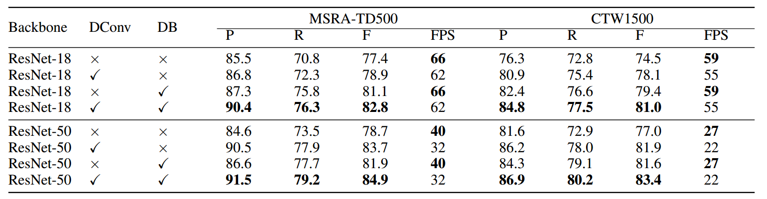
论文中指标结果：

可以看出变形卷积和阈值图对整个性能都有比较大的促进作用。

image.png-99.9kB

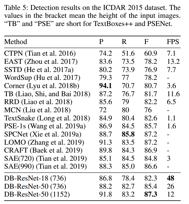
测试icdar2015数据结果：

image.png-199.6kB

lexi_qi

关注

15
点赞
踩
49

收藏

觉得还不错? 一键收藏
2
评论
DBNet详解

目录创新点算法的整体架构自适应阈值（Adaptive threshhold）二值化标准二值化可微二值(differentiable Binarization)直观展示可形变卷积（Deformable convolution）标签的生成PSENet标签生成DBNet标签生成损失函数后处理代码阅读数据预处理入口AugmentDetectionData（数据增强类）RandomCropData（数据裁剪类）MakeICDARData（数据重新组织类）MakeSegDetectionData(生成概率图和对应ma
复制链接

扫一扫