DBNet源码——超详细图解

最新推荐文章于 2024-12-31 21:23:25 发布

凯尔哥

最新推荐文章于 2024-12-31 21:23:25 发布

阅读量2.4k

点赞数 25

分类专栏：深度学习源码图解系列文章标签：深度学习 ocr

本文链接：https://blog.csdn.net/weixin_43507865/article/details/136671486

版权

深度学习源码图解系列专栏收录该内容

5 篇文章

订阅专栏

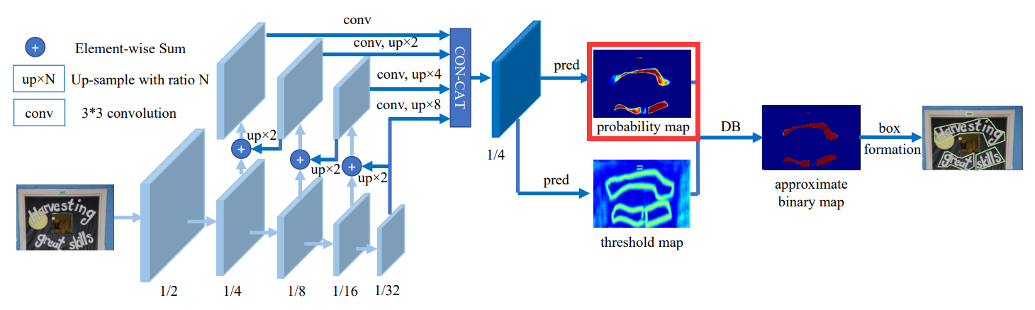
论文地址：https://arxiv.org/pdf/1911.08947.pdf

模型代码：GitHub - WenmuZhou/DBNet.pytorch: A pytorch re-implementation of Real-time Scene Text Detection with Differentiable Binarization

1. 准备训练数据

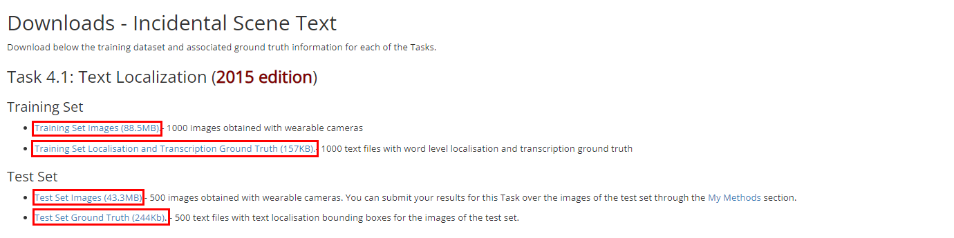
1.1. 下载数据

数据下载地址：Downloads - Incidental Scene Text - Robust Reading Competition

1.2. 准备数据

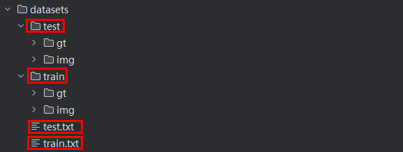
下载之后又 4 个压缩包，如下所示：

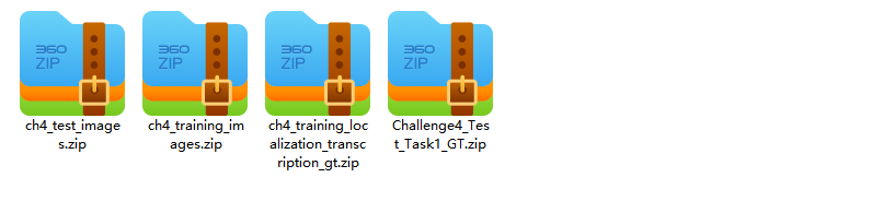
分别将四个压缩包解压

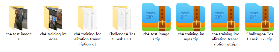
新建 train 和 test 文件夹

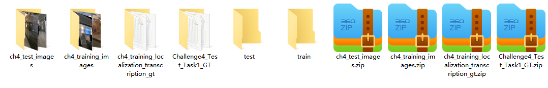
将ch4_training_images、ch4_training_localization_transcription_gt 文件夹移动到 train 文件夹内，然后将ch4_training_images 文件夹重新命名为 img，将ch4_training_localization_transcription_gt 文件夹重命名为 gt；

将ch4_test_images、Challenge4_Test_Task1_GT 文件夹移动到 test 文件夹内，然后将ch4_test_images 文件夹重新命名为 img，将Challenge4_Test_Task1_GT 文件夹重命名为 gt。

使用如下代码准备 train.txt 和 test.txt。需要将路径替换为自己的路径。

import os
def get_images(img_path):
    '''
    find image files in data path
    :return: list of files found
    '''
    img_path = os.path.abspath(img_path)
    files = []
    exts = ['jpg', 'png', 'jpeg', 'JPG', 'PNG']
    for parent, dirnames, filenames in os.walk(img_path):
        for filename in filenames:
            for ext in exts:
                if filename.endswith(ext):
                    files.append(os.path.join(parent, filename))
                    break
    print('Find {} images'.format(len(files)))
    return sorted(files)
    
def get_txts(txt_path):
    '''
    find gt files in data path
    :return: list of files found
    '''
    txt_path = os.path.abspath(txt_path)
    files = []
    exts = ['txt']
    for parent, dirnames, filenames in os.walk(txt_path):
        for filename in filenames:
            for ext in exts:
                if filename.endswith(ext):
                    files.append(os.path.join(parent, filename))
                    break
    print('Find {} txts'.format(len(files)))
    return sorted(files)    

if __name__ == '__main__':
    #img_path = './train/img'	
    img_path = './test/img'
    files = get_images(img_path)
    #txt_path = './train/gt'
    txt_path = './test/gt'
    txts = get_txts(txt_path)
    n = len(files)
    assert len(files) == len(txts)
    with open('test.txt', 'w') as f:
        for i in range(n):
            line = files[i] + '\t' + txts[i] + '\n'
            f.write(line)
    
    print('dataset generated ^_^ ')

将生成好的 train.txt、test.txt、train 文件夹、test 文件夹放到项目的 datasets 文件夹下

2. 制作标签

2.1. 制作threshold map 标签

data_loader/modules/make_border_map.py

2.1.1. 程序入口 if name == 'main'

if __name__ == '__main__':
    import numpy as np
    make_border_map = MakeBorderMap()	# 实例化MakeBorderMap对象
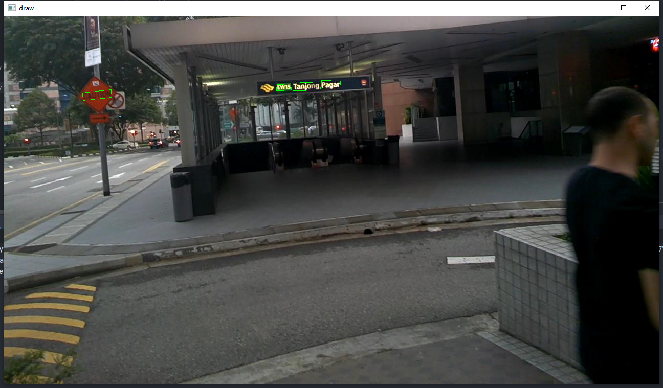
    img = cv2.imread("../../datasets/train/img/img_41.jpg")	# 随机选取一张图片做演示
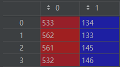
    # shape (4, 4, 2)，表示该张图片上有4个文本区域，每个文本区域有4个坐标(x,y)
    points = np.array([[[533, 134], [562, 133], [561, 145], [532, 146]],
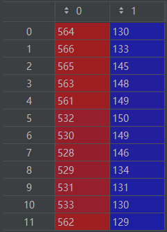
                       [[564, 131], [617, 129], [617, 145], [564, 146]],
                       [[620, 126], [657, 127], [656, 143], [618, 143]],
                       [[153, 150], [209, 144], [210, 159], [154, 165]]])
    draw_img = img.copy()
    # 可视化一下该图片上的文本区域
    for pt in points:
        # 画多边形
        cv2.polylines(draw_img, [pt], True, color=(0, 255, 0))
    # 显示绘制多边形后的结果
    cv2.imshow("draw", draw_img)
    cv2.waitKey(0)
    cv2.destroyAllWindows()
    # 该图片上的文本内容
    texts = ['EW15', 'Tanjong', 'Pagar', 'CAUTION']
    # 是否要忽略掉该文本区域。如果文本区域过小，那么需要忽略，后面的代码有解释。
    ignore_tags = [False, False, False, False]
    data = {"img": img, "img_41": "img_41", "text_polys": points, "texts": texts, "ignore_tags": ignore_tags}
    # 实际构造threshold map 标签
    data = make_border_map(data)
    print(data)

img_41.jpg的文本区域可视化的结果如下：

2.1.2. 调用make_border_map对象

make_border_map.py

def __call__(self, data: dict) -> dict:
	"""
	从scales中随机选择一个尺度，对图片和文本框进行缩放
	:param data: {'img':,'text_polys':,'texts':,'ignore_tags':}
	:return:
	"""
    # 需要标注的图片
	im = data['img']
    # 图片上的实际的文本区域
	text_polys = data['text_polys']
    # 是否需要忽略掉该文本区域
	ignore_tags = data['ignore_tags']
	# canvas，即最后的threshold_map，其shape为图片的实际大小，用0初始化
	canvas = np.zeros(im.shape[:2], dtype=np.float32)
    # mask：在计算机图形领域，"mask" 也可以指遮罩，一种用于控制图像中某些区域可见性的图形。
    # shape为图片的实际大小，用0初始化
	mask = np.zeros(im.shape[:2], dtype=np.float32)

	for i in range(len(text_polys)):    # 文本框的个数
        # 如果该文本区域需要忽略，则跳过
		if ignore_tags[i]:
			continue
        # 实际构造标签的方法
		self.draw_border_map(text_polys[i], canvas, mask=mask)
	canvas = canvas * (self.thresh_max - self.thresh_min) + self.thresh_min

	data['threshold_map'] = canvas
	data['threshold_mask'] = mask
	return data

canvas/gt的初始状态

其中，h表示原图的高度，w表示原图的宽度

mask的初始状态

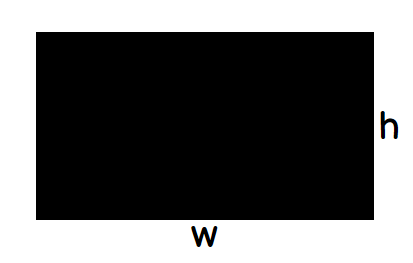
其中，h表示原图的高度，w表示原图的宽度

2.1.3. 进入draw_border_map()方法

make_border_map.py

def draw_border_map(self, polygon, canvas, mask):
	polygon = np.array(polygon) # (4,2)
	assert polygon.ndim == 2
	assert polygon.shape[1] == 2
	#构造多边形对象
	"""
    Example
    -------
    Create a square polygon with no holes
    
      >>> coords = ((0., 0.), (0., 1.), (1., 1.), (1., 0.), (0., 0.))
      >>> polygon = Polygon(coords)
      >>> polygon.area
      1.0
    """
	polygon_shape = Polygon(polygon)
    # 多边形面积小于0，直接return
	if polygon_shape.area <= 0: 
		return
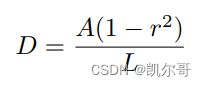
    # 计算膨胀和收缩的距离，该公式为论文中的公式
	distance = polygon_shape.area * (1 - np.power(self.shrink_ratio, 2)) / polygon_shape.length     
	subject = (tuple(l) for l in polygon)
    # pyclipper.PyclipperOffset()：图形内缩，可以将多边形向内缩放n个距离后的图形
	padding = pyclipper.PyclipperOffset() 
	padding.AddPath(subject, pyclipper.JT_ROUND,
					pyclipper.ET_CLOSEDPOLYGON)
    # 计算出来的distance是正数，所以是膨胀边框
    # padded_polygon shape：[n, 2]
	padded_polygon = np.array(padding.Execute(distance)[0])     
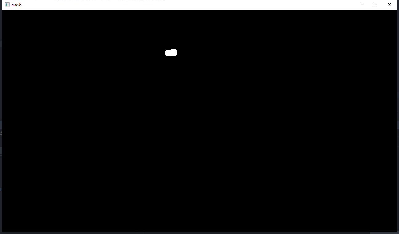
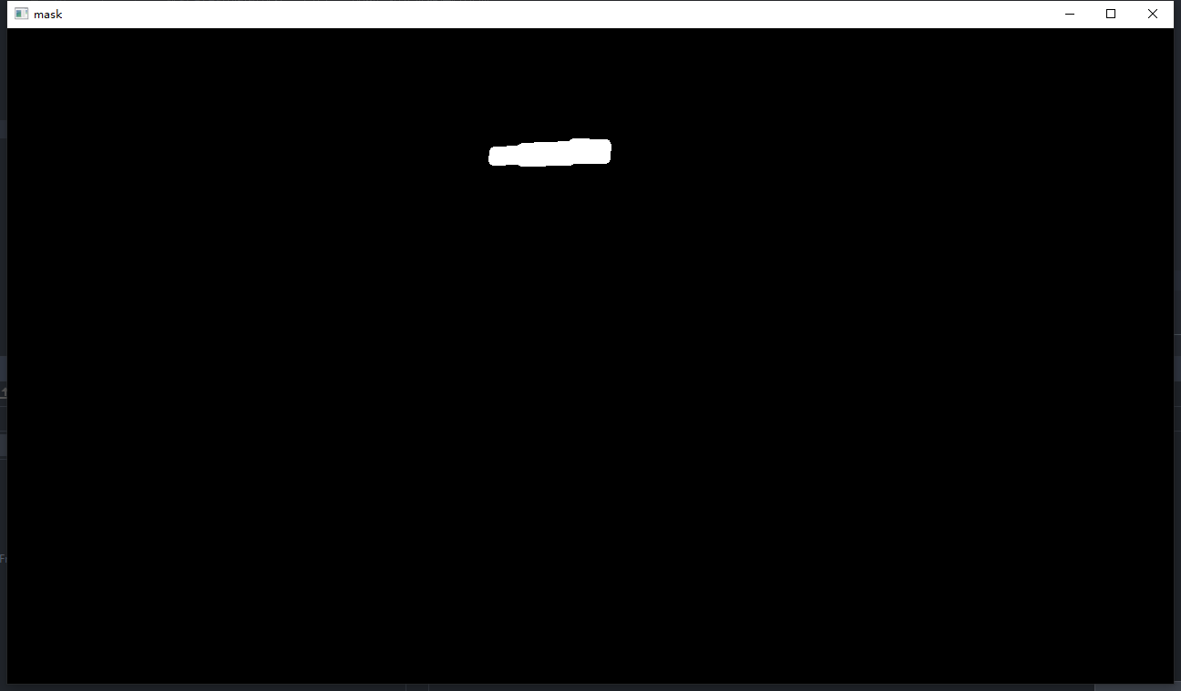
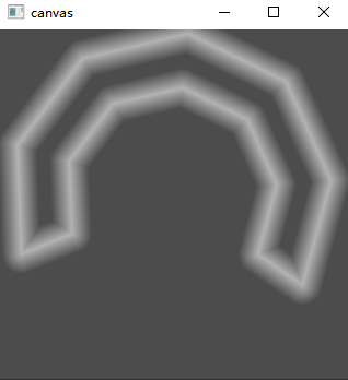
    # 用计算出来的膨胀多边形填充mask
	cv2.fillPoly(mask, [padded_polygon.astype(np.int32)], (255, 255, 255))
	plt.imshow(mask)
	plt.show()
	# cv2.imshow("mask", mask)
	# cv2.waitKey(0)
	# # closing all open windows
	# cv2.destroyAllWindows()

	xmin = padded_polygon[:, 0].min()   # x坐标的最小值
	xmax = padded_polygon[:, 0].max()   # x坐标的最大值
	ymin = padded_polygon[:, 1].min()   # y坐标的最小值
	ymax = padded_polygon[:, 1].max()   # y坐标的最大值
	width = xmax - xmin + 1             # 宽
	height = ymax - ymin + 1            # 高
    # 将多边形相对于原始图片的坐标转换为多边形相对于膨胀后的多边形的坐标
	polygon[:, 0] = polygon[:, 0] - xmin
	polygon[:, 1] = polygon[:, 1] - ymin

	xs = np.broadcast_to(
		np.linspace(0, width - 1, num=width).reshape(1, width), (height, width))
	ys = np.broadcast_to(
		np.linspace(0, height - 1, num=height).reshape(height, 1), (height, width))
	# (4,22,39)  定义一个distance_map 用于保存每一个点到每一条边的距离
	distance_map = np.zeros(
		(polygon.shape[0], height, width), dtype=np.float32)
    # 遍历每一个文本框，计算该文本框同膨胀后多边形每一个边的距离
	for i in range(polygon.shape[0]):
		j = (i + 1) % polygon.shape[0]
        # 核心方法：计算扩张后的边界框内所有点到该条边的距离
		absolute_distance = self.distance(xs, ys, polygon[i], polygon[j]) 
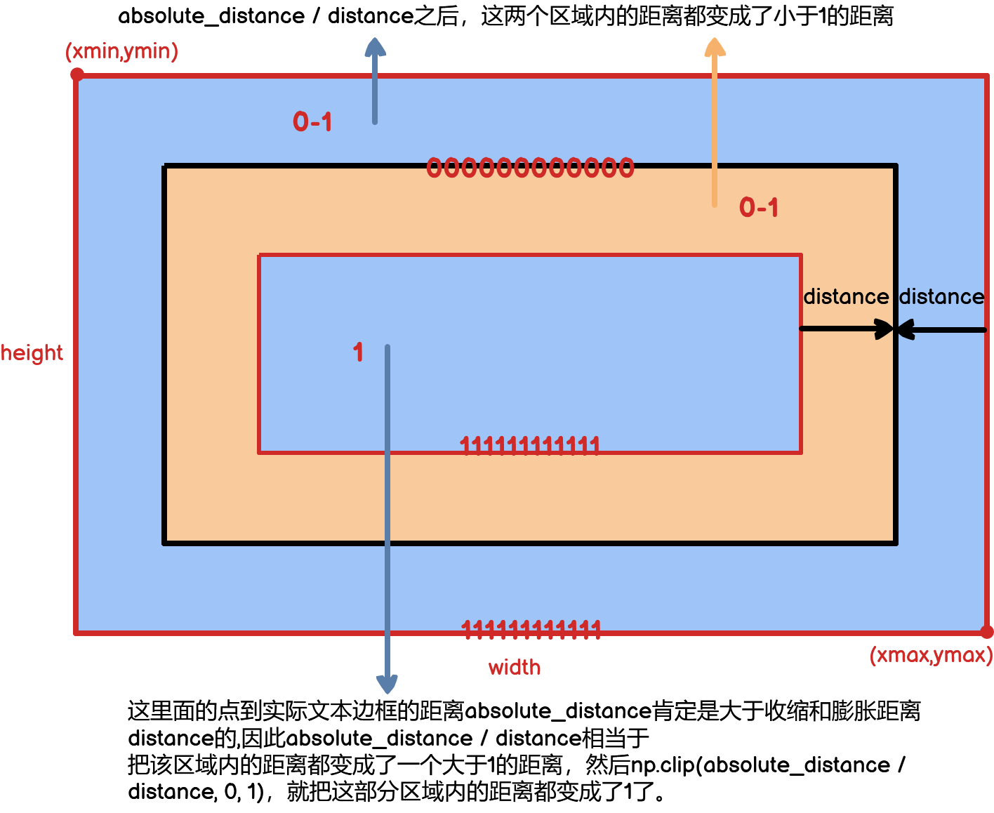
        # 将得到的距离除以扩张的偏移量进行归一化，并且将值限制在[0,1]以内
		distance_map[i] = np.clip(absolute_distance / distance, 0, 1) 
    # 只保留某个点到距离最近的边的距离
	distance_map = distance_map.min(axis=0)  
    
	# 保证xmin，xmax，ymin，ymax的坐标在canvas的范围内
	xmin_valid = min(max(0, xmin), canvas.shape[1] - 1)
	xmax_valid = min(max(0, xmax), canvas.shape[1] - 1)
	ymin_valid = min(max(0, ymin), canvas.shape[0] - 1)
	ymax_valid = min(max(0, ymax), canvas.shape[0] - 1)
    
	canvas[ymin_valid:ymax_valid + 1, xmin_valid:xmax_valid + 1] = np.fmax(
		1 - distance_map[
			ymin_valid - ymin:ymax_valid - ymax + height,
			xmin_valid - xmin:xmax_valid - xmax + width],
		canvas[ymin_valid:ymax_valid + 1, xmin_valid:xmax_valid + 1])

上面的代码中，

polygon = np.array(polygon)

上面的代码中，

distance = polygon_shape.area * (1 - np.power(self.shrink_ratio, 2)) / polygon_shape.length用于计算膨胀和收缩的距离，其计算公式来源于论文

上面代码中，

padded_polygon = np.array(padding.Execute(distance)[0])

上面的代码中，

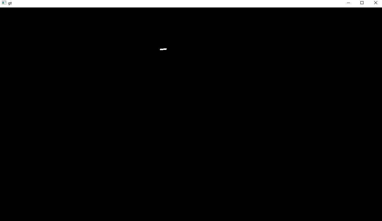
cv2.fillPoly(mask, [padded_polygon.astype(np.int32)], 1)的结果可视化如下：

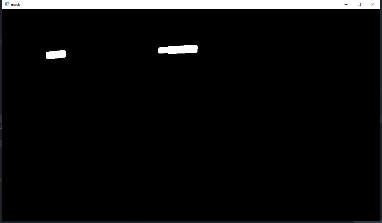
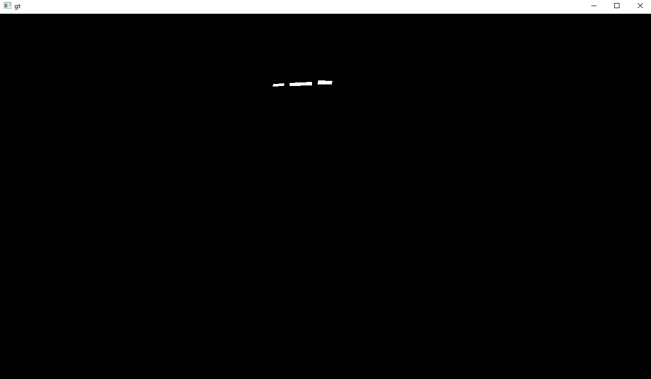
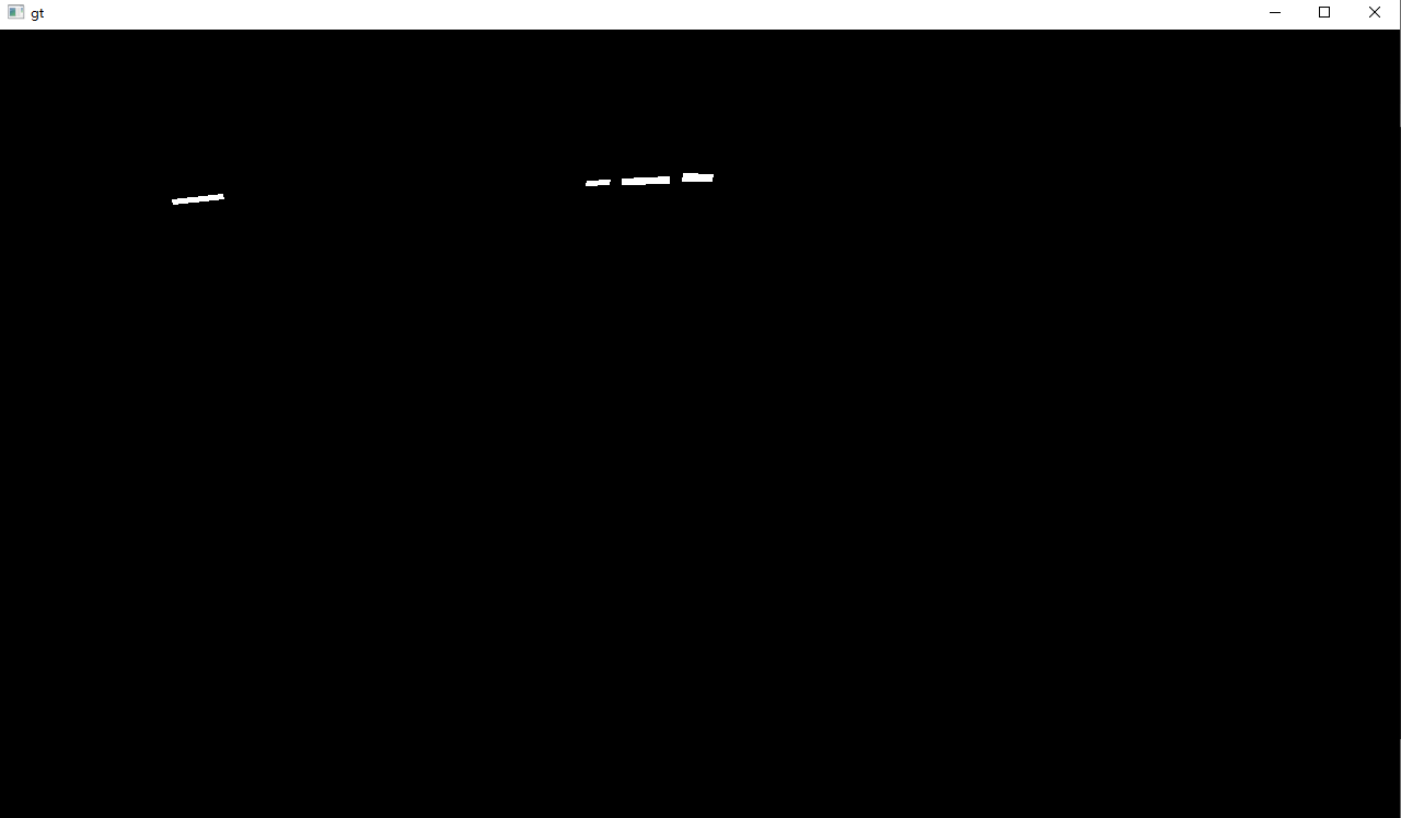
因为每次传入的mask是之前的mask(def draw_border_map(self, polygon, canvas, mask))，所以每次会在之前的mask上继续填充多边形。

第一个文本区域

第一、二个文本区域

第一、二、三个文本区域

第一、二、三、四个文本区域

上面代码中，

xmin = padded_polygon[:, 0].min()   # x坐标的最小值
xmax = padded_polygon[:, 0].max()   # x坐标的最大值
ymin = padded_polygon[:, 1].min()   # y坐标的最小值
ymax = padded_polygon[:, 1].max()   # y坐标的最大值
width = xmax - xmin + 1             # 膨胀之后，文字框的宽度
height = ymax - ymin + 1            # 膨胀之后，文字框的高度

由于求出来的膨胀多边形可能有多个坐标点，因此，在x和y方向只选取一个最小值和一个最小值。

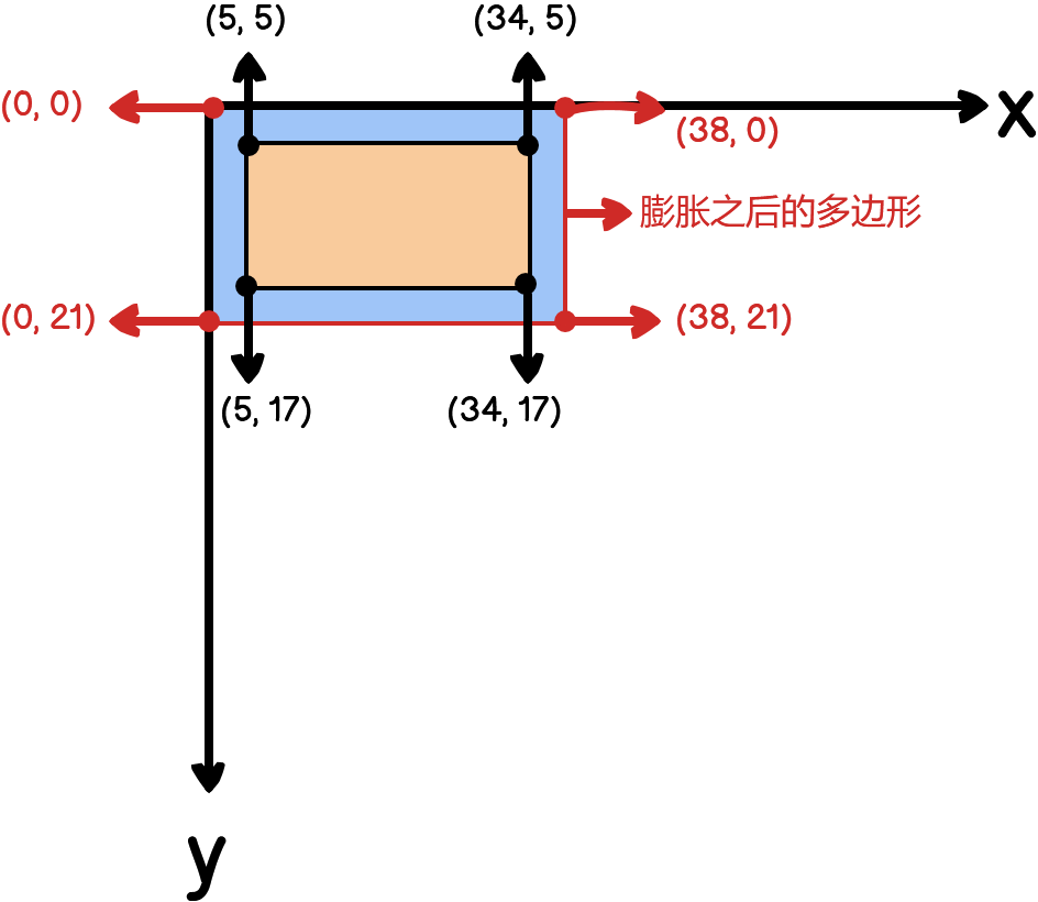
polygon[:, 0] = polygon[:, 0] - xmin
polygon[:, 1] = polygon[:, 1] - ymin

这两行代码的作用用可视化的方式解释如下：

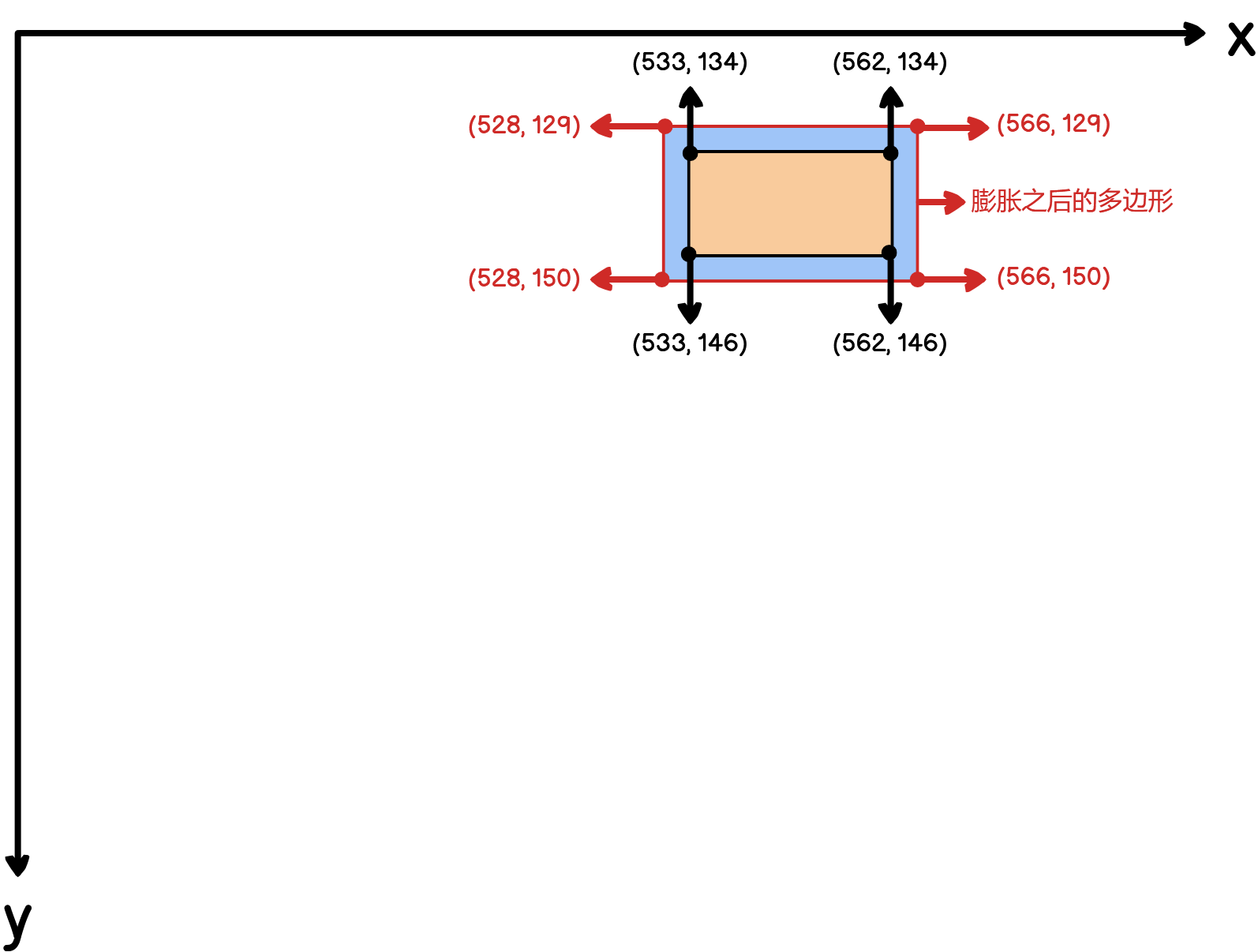
上面图中的文本框坐标值是相对于原始图像的，现在要将其转换为相对于膨胀之后的多边形的坐标，如下图所示：

上面代码中，

xs = np.broadcast_to(
    np.linspace(0, width - 1, num=width).reshape(1, width), (height, width))
ys = np.broadcast_to(
    np.linspace(0, height - 1, num=height).reshape(height, 1), (height, width))

用可视化的方式解释如下：

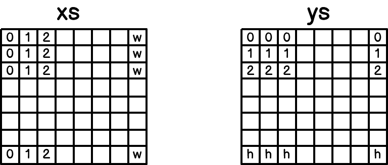
定义xs和ys的目的是为了计算每一个点到原始文本框每一条边的距离，具体体现在absolute_distance = self.distance(xs, ys, polygon[i], polygon[j])这一行代码

2.1.4. 进入distance()方法

def distance(self, xs, ys, point_1, point_2):
 	'''
 	compute the distance from point to a line
 	ys: coordinates in the first axis
 	xs: coordinates in the second axis
 	point_1, point_2: (x, y), the end of the line
 	'''
 	# height, width = xs.shape[:2]
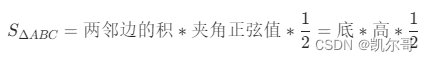
 	square_distance_1 = np.square(xs - point_1[0]) + np.square(ys - point_1[1])
 	square_distance_2 = np.square(xs - point_2[0]) + np.square(ys - point_2[1])
     # 文本框一条边的长度
 	square_distance = np.square(point_1[0] - point_2[0]) + np.square(point_1[1] - point_2[1])   
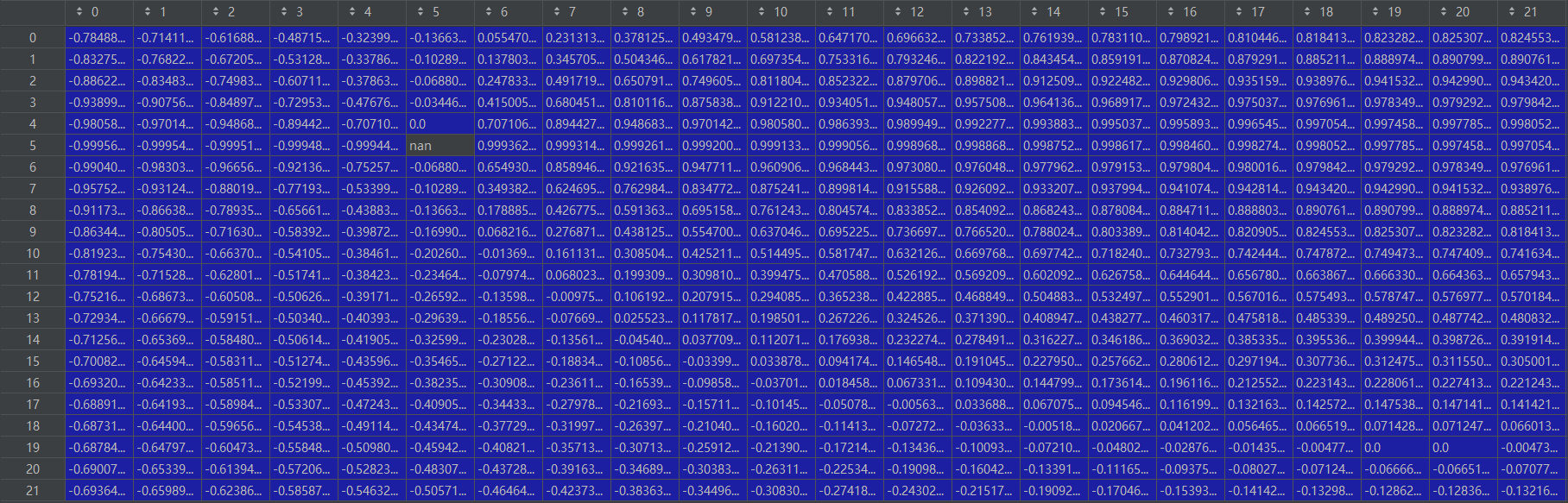
 	# 余弦距离, shape:(22*39)
 	cosin = (square_distance - square_distance_1 - square_distance_2) / (2 * np.sqrt(square_distance_1 * square_distance_2))
 	square_sin = 1 - np.square(cosin)       # sin² x + cos² x = 1
 	square_sin = np.nan_to_num(square_sin)  # 用0替代nan值
 
 	result = np.sqrt(square_distance_1 * square_distance_2 * square_sin / square_distance)
     # 不知道这行代码的意思？如果有理解的大佬还请解释一下
 	result[cosin < 0] = np.sqrt(np.fmin(square_distance_1, square_distance_2))[cosin < 0]
 	# self.extend_line(point_1, point_2, result)
 	return result

上面代码中，

# 距离的平方
square_distance_1 = np.square(xs - point_1[0]) + np.square(ys - point_1[1])
square_distance_2 = np.square(xs - point_2[0]) + np.square(ys - point_2[1])
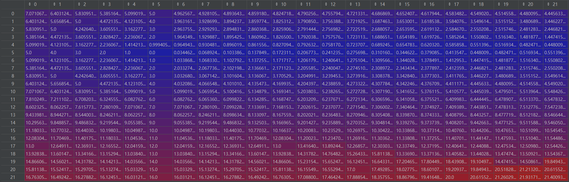
square_distance = np.square(point_1[0] - point_2[0]) + np.square(point_1[1] - point_2[1])

用可视化的方式解释如下：

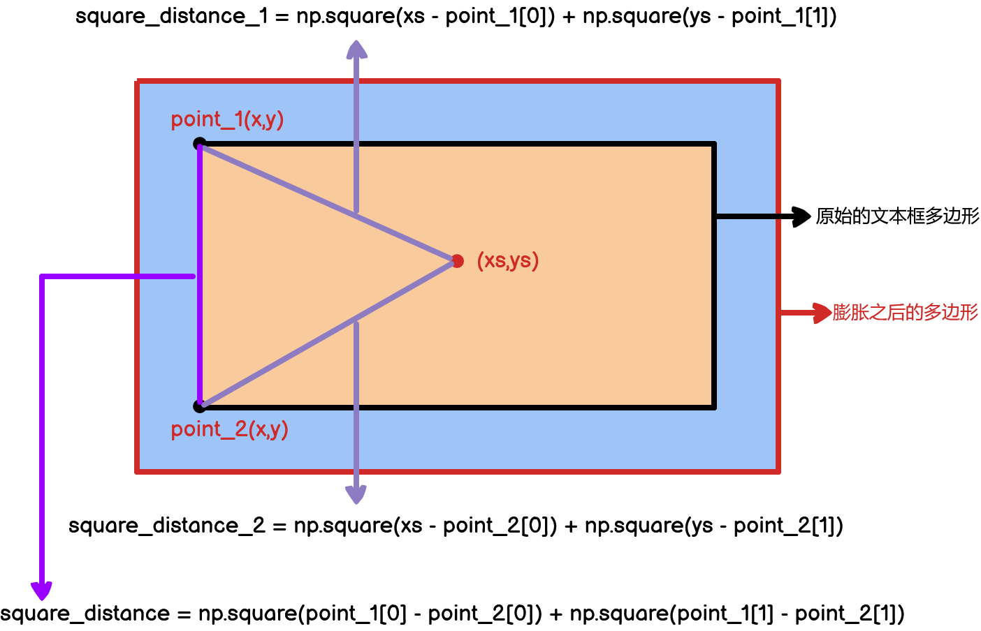
result的shape为膨胀之后的多边形的shape，表示每一个点到一条边的距离。

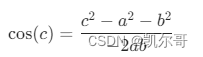
上面代码中，

cosin = (square_distance - square_distance_1 - square_distance_2) / (2 * np.sqrt(square_distance_1 * square_distance_2))

用到了余弦定理，公式如下：

变换得到，

在三角学中，余弦函数的取值范围是在区间 [−1,1] 内。具体来说：

对于锐角（角度在0-90度之间），余弦值是正的，范围在 [0,1]；
对于直角（角度为90度），余弦值为零；
对于钝角（角度在90-180度之间），余弦值是负的，范围在 [−1,0)。

上面的公式少了一个负号，因此，结果正好相反。

cosin 的结果如下：

上面的代码中，

square_sin = 1 - np.square(cosin)

上面的代码中，

result = np.sqrt(square_distance_1 * square_distance_2 * square_sin / square_distance)

这行代码来源于，三角形的面积公式，对于任意三角形，其面积的计算公式如下：

根据上面的公式，可得出result = np.sqrt(square_distance_1) * np.sqrt(square_distance_2) * np.sqrt(square_sin) * 0.5/ np.sqrt(square_distance) * 0.5 = np.sqrt(square_distance_1 * square_distance_2 * square_sin / square_distance)

result 的结果如下：

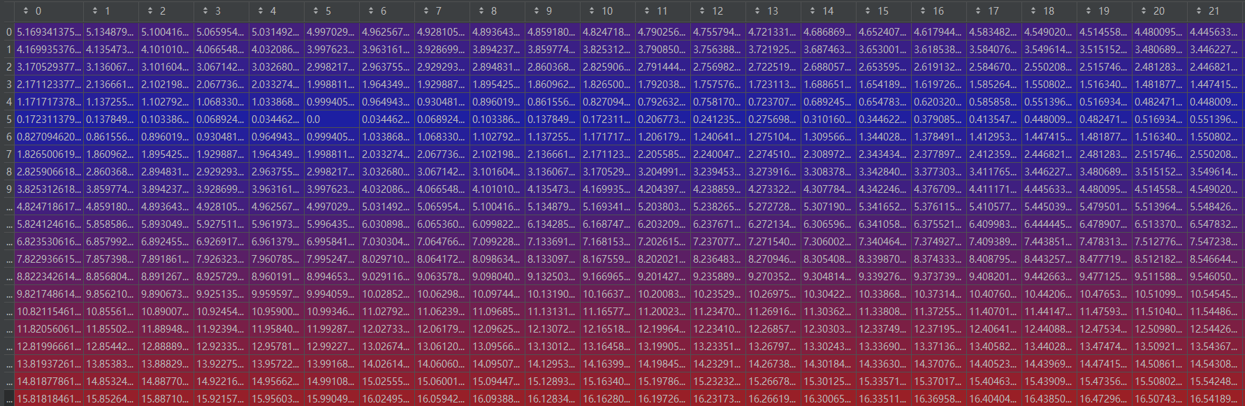
上面的代码中，

result[cosin < 0] = np.sqrt(np.fmin(square_distance_1, square_distance_2))[cosin < 0]

网上说的是锐角就选择最短的哪条边作为点到线段的距离，对比一下有这行代码和没有这段代码的区别

有这行代码

没有这行代码

很明显有这行代码的效果更好。

更新之后的 result 的结果如下：

2.1.5. 再退回到draw_border_map()方法

来到下面这行代码

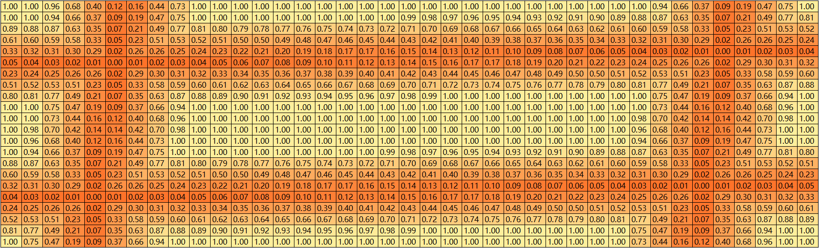
distance_map[i] = np.clip(absolute_distance / distance, 0, 1)

用可视化的方式解释如下：

再继续，来到下面这行代码

distance_map = distance_map.min(axis=0)  # 只保留某个点到距离最近的边的距离

到这里，已经求出了每一个点到每一条边的距离，这时候只选最近的那个距离，distance_map的shape就变为了(height, width)，即膨胀之后的多边形的高度和宽度。

再往下，

canvas[ymin_valid:ymax_valid + 1, xmin_valid:xmax_valid + 1] = np.fmax(
	1 - distance_map[
		ymin_valid - ymin:ymax_valid - ymax + height,
		xmin_valid - xmin:xmax_valid - xmax + width],
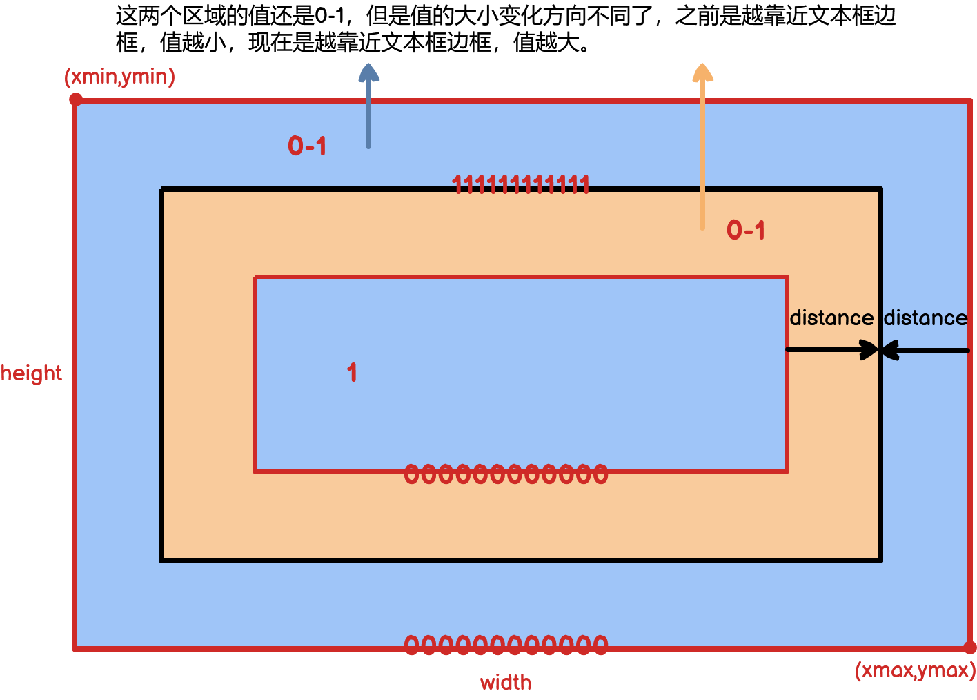
	canvas[ymin_valid:ymax_valid + 1, xmin_valid:xmax_valid + 1])

这段代码其实就是在往canvas图像上填充值了，用1减去distance_map上每一个像素点的值，相当于把距离做了一下变化，之前最大的距离1，现在变成了0，之前最小的距离0，现在变成了1。然后再同原始的canvas图像上的像素点(初始的时候都是0)计算最大值。

2.1.6. 最后，退回到make_border_map对象的调用方法

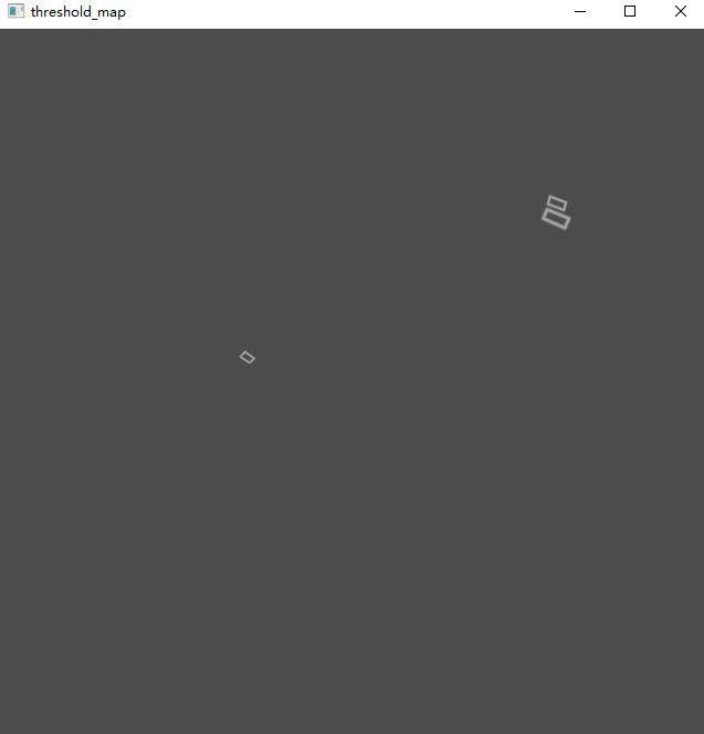
来到这行代码，

canvas = canvas * (self.thresh_max - self.thresh_min) + self.thresh_min

该行代码的作用就是将canvas里面的值压缩到self.thresh_min到self.thresh_max之间，即0.3-0.7。

可视化结果如下：

到这里，threshold_map的标签就制作好了。

另外，如果是针对多边形标注，代码是一样的，下面是对印章的标注结果

2.2. 制作probability map 标签

data_loader/modules/make_shrink_map.py

还是以`../../datasets/train/img/img_41.jpg`这张图片为例

2.2.1. 调用MakeShrinkMap对象

def __call__(self, data: dict) -> dict:
	"""
	从scales中随机选择一个尺度，对图片和文本框进行缩放
	:param data: {'img':,'text_polys':,'texts':,'ignore_tags':}
	:return:
	"""
	image = data['img']
	text_polys = data['text_polys']
	ignore_tags = data['ignore_tags']

	h, w = image.shape[:2]
    # 验证文本框坐标的有效性以及变换坐标顺序
	text_polys, ignore_tags = self.validate_polygons(text_polys, ignore_tags, h, w)
    # 真实标签
	gt = np.zeros((h, w), dtype=np.float32)
	mask = np.ones((h, w), dtype=np.float32)
	for i in range(len(text_polys)):
		polygon = text_polys[i]
        # 计算文本框的高度
		height = max(polygon[:, 1]) - min(polygon[:, 1])
        # 计算文本框的宽度
		width = max(polygon[:, 0]) - min(polygon[:, 0])
        # 如果需要忽略掉这个文本框或者该文本框的大小小于self.min_text_size，那么在mask上用黑色填充
		if ignore_tags[i] or min(height, width) < self.min_text_size:
            # 在mask上填充
			cv2.fillPoly(mask, polygon.astype(np.int32)[np.newaxis, :, :], 0)
			ignore_tags[i] = True
		else:
            # 完成收缩的方法
			shrinked = self.shrink_func(polygon, self.shrink_ratio)
            # 如果最后没有收缩
			if shrinked.size == 0:
                # 在mask上用黑色填充
				cv2.fillPoly(mask, polygon.astype(np.int32)[np.newaxis, :, :], 0)
				ignore_tags[i] = True
				continue
			cv2.fillPoly(gt, [shrinked.astype(np.int32)], 1)

	data['shrink_map'] = gt
	data['shrink_mask'] = mask
	return data

上面代码中，

text_polys, ignore_tags = self.validate_polygons(text_polys, ignore_tags, h, w)

这行代码的作用是验证文本框的边框是否是超出了原始图片的范围，并且将文本框的坐标顺序进行了一个调换。例如，`[[533, 134], [562, 133], [561, 145], [532, 146]]`这个文本框坐标调换顺序之后变为`[[532, 146], [561, 145], [562, 133], [533, 134]]`。

接着往下，

gt = np.zeros((h, w), dtype=np.float32)
mask = np.ones((h, w), dtype=np.float32)

gt的可视化结果如下：

mask的可视化结果如下：

接着往下

shrinked = self.shrink_func(polygon, self.shrink_ratio)

这行代码的作用是完成边框的收缩

2.2.2. 进入shrink_func()方法

def shrink_polygon_pyclipper(polygon, shrink_ratio):
    from shapely.geometry import Polygon
    import pyclipper
    polygon_shape = Polygon(polygon)
    # 计算需要缩放的偏移量,其公式来源于论文
    distance = polygon_shape.area * (1 - np.power(shrink_ratio, 2)) / polygon_shape.length  
    subject = [tuple(l) for l in polygon]
    padding = pyclipper.PyclipperOffset()
    padding.AddPath(subject, pyclipper.JT_ROUND, pyclipper.ET_CLOSEDPOLYGON)
    # 缩放边框
    shrinked = padding.Execute(-distance)
    if shrinked == []:
        shrinked = np.array(shrinked)
    else:
        shrinked = np.array(shrinked[0]).reshape(-1, 2)
    return shrinked

上面代码中，

distance = polygon_shape.area * (1 - np.power(shrink_ratio, 2)) / polygon_shape.length

该行代码的作用是计算需要缩放的偏移量，其计算公式如下：

2.2.3. 最后，回到MakeShrinkMap对象

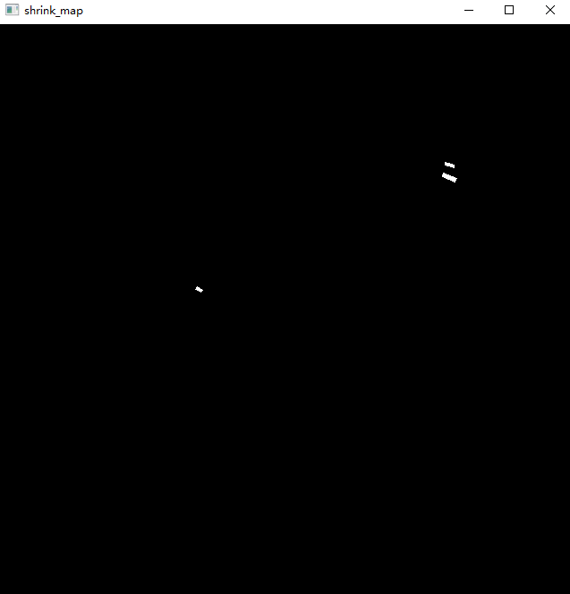
来到这行代码

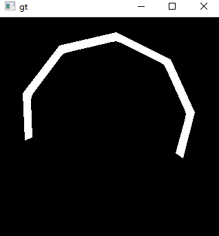
cv2.fillPoly(gt, [shrinked.astype(np.int32)], 1)

这行代码的作用就是在gt上用白色填充缩放后的多边形，可视化效果如下：

第一个文本框的缩放gt

第一个和第二个文本框的缩放gt

第一个、第二个和第三个文本框的缩放gt

第一个、第二个、第三个和第四个文本框的缩放gt

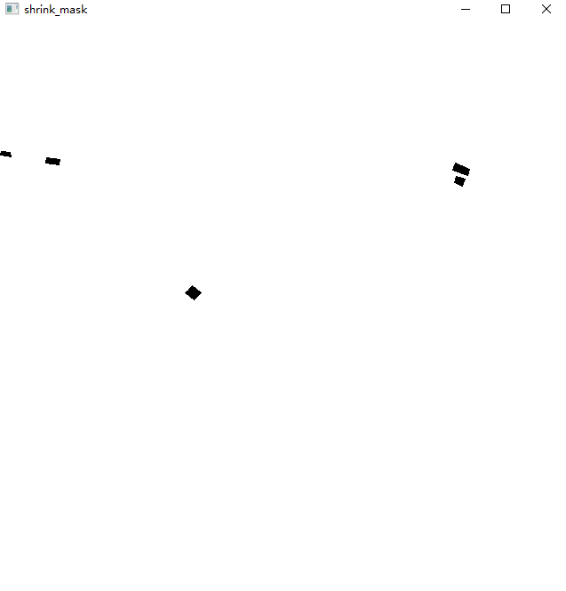
而mask自始至终都是全白色，没有任何变化，如下图所示：

到这里，probability map的标签就制作好了。

另外，如果是针对多边形标注，代码是一样的，下面是对印章的标注结果

3. 训练模型

models/model.py

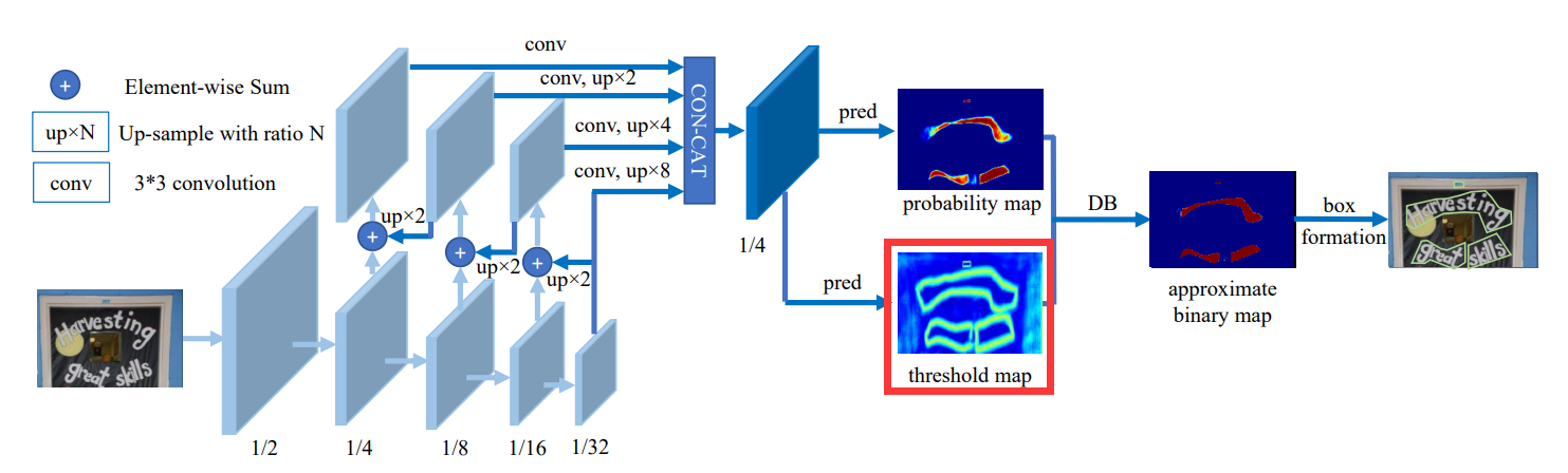
3.1. backbone

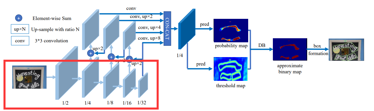
基础网络：ResNet18
核心代码：self.backbone = build_backbone(backbone_type, **model_config.backbone)

3.1.1. 进入 model.py

class Model(nn.Module):
    def __init__(self, model_config: dict):
        """
        PANnet
        :param model_config: 模型配置
        """
        super().__init__()
        model_config = Dict(model_config)
        backbone_type = model_config.backbone.pop('type')
        neck_type = model_config.neck.pop('type')
        head_type = model_config.head.pop('type')
        # 构建backbone网络
        self.backbone = build_backbone(backbone_type, **model_config.backbone)
        # 构建neck网络
        self.neck = build_neck(neck_type, in_channels=self.backbone.out_channels, **model_config.neck)
        # 构建head网络
        self.head = build_head(head_type, in_channels=self.neck.out_channels, **model_config.head)
        self.name = f'{backbone_type}_{neck_type}_{head_type}'

    def forward(self, x):
        _, _, H, W = x.size()
        backbone_out = self.backbone(x)
        neck_out = self.neck(backbone_out)
        y = self.head(neck_out)
        y = F.interpolate(y, size=(H, W), mode='bilinear', align_corners=True)
        return y

3.1.2. 进入build_backbone()方法

def build_backbone(backbone_name, **kwargs):
    assert backbone_name in support_backbone, f'all support backbone is {support_backbone}'
    backbone = eval(backbone_name)(**kwargs)
    return backbone

3.1.3. 跳转到resnet.py中的resnet18()方法

def resnet18(pretrained=True, **kwargs):
    """Constructs a ResNet-18 model.
    Args:
        pretrained (bool): If True, returns a model pre-trained on ImageNet
    """
    # 构造ResNet18模型
    model = ResNet(BasicBlock, [2, 2, 2, 2], **kwargs)
    if pretrained:
        assert kwargs['in_channels'] == 3, 'in_channels must be 3 whem pretrained is True'
        print('load from imagenet')
        model.load_state_dict(model_zoo.load_url(model_urls['resnet18']), strict=False)
    return model

3.1.4. 跳转到resnet.py中的ResNet类

class ResNet(nn.Module):
    def __init__(self, block, layers, in_channels=3, dcn=None):
        self.dcn = dcn			# 是否使用反卷积
        self.inplanes = 64		# 每一层输入的channel数
        super(ResNet, self).__init__()
        self.out_channels = []	# 保存好输出的channel
        # 定义卷积操作
        self.conv1 = nn.Conv2d(in_channels, 64, kernel_size=7, stride=2, padding=3,
                               bias=False)
        # 定义BN操作
        self.bn1 = BatchNorm2d(64)
        # 定义激活操作
        self.relu = nn.ReLU(inplace=True)
        # 定义MaxPooling操作
        self.maxpool = nn.MaxPool2d(kernel_size=3, stride=2, padding=1)
        # layers = [2, 2, 2, 2]
        # 每一特征层由两个BasicBlock组成
        self.layer1 = self._make_layer(block, 64, layers[0])	
        # 这里的第一个BasicBlock需要先进行下采样，将上一一个layer输出的channel 由64变为128
        self.layer2 = self._make_layer(block, 128, layers[1], stride=2, dcn=dcn)
        self.layer3 = self._make_layer(block, 256, layers[2], stride=2, dcn=dcn)
        self.layer4 = self._make_layer(block, 512, layers[3], stride=2, dcn=dcn)
        
		# self.modules()保存的是模型结构中所有的操作，包括卷积、池化等。self.modules()采用深度优先遍历的方式，存储了net的所有模块，参考博客：https://blog.csdn.net/dss_dssssd/article/details/83958518
        for m in self.modules():
            # 如果是卷积
            if isinstance(m, nn.Conv2d):		# 卷积核w参数初始化
                n = m.kernel_size[0] * m.kernel_size[1] * m.out_channels
                m.weight.data.normal_(0, math.sqrt(2. / n))
            # 如果是BN
            elif isinstance(m, BatchNorm2d):	# BN参数初始化
                m.weight.data.fill_(1)
                m.bias.data.zero_()
        if self.dcn is not None:
            for m in self.modules():
                if isinstance(m, Bottleneck) or isinstance(m, BasicBlock):
                    if hasattr(m, 'conv2_offset'):
                        constant_init(m.conv2_offset, 0)
    def _make_layer(self, block, planes, blocks, stride=1, dcn=None):
            # 构造一个网络层
            downsample = None
            # 是否需要下采样，在 stride != 1 和 输入维度同输出维度不一致  这两种情况下需要进行下采样
            if stride != 1 or self.inplanes != planes * block.expansion:
                downsample = nn.Sequential(
                    nn.Conv2d(self.inplanes, planes * block.expansion,
                              kernel_size=1, stride=stride, bias=False),
                    BatchNorm2d(planes * block.expansion),
                )
    
            layers = []
            # 构建一个残差块，其中包括3*3的卷积、BN和激活
            layers.append(block(self.inplanes, planes, stride, downsample, dcn=dcn))
            #  修改输入的维度
            self.inplanes = planes * block.expansion
            for i in range(1, blocks):
                layers.append(block(self.inplanes, planes, dcn=dcn))
            self.out_channels.append(planes * block.expansion)
            return nn.Sequential(*layers)	# nn.Sequential用法，这里传入的是一个list

    def forward(self, x):
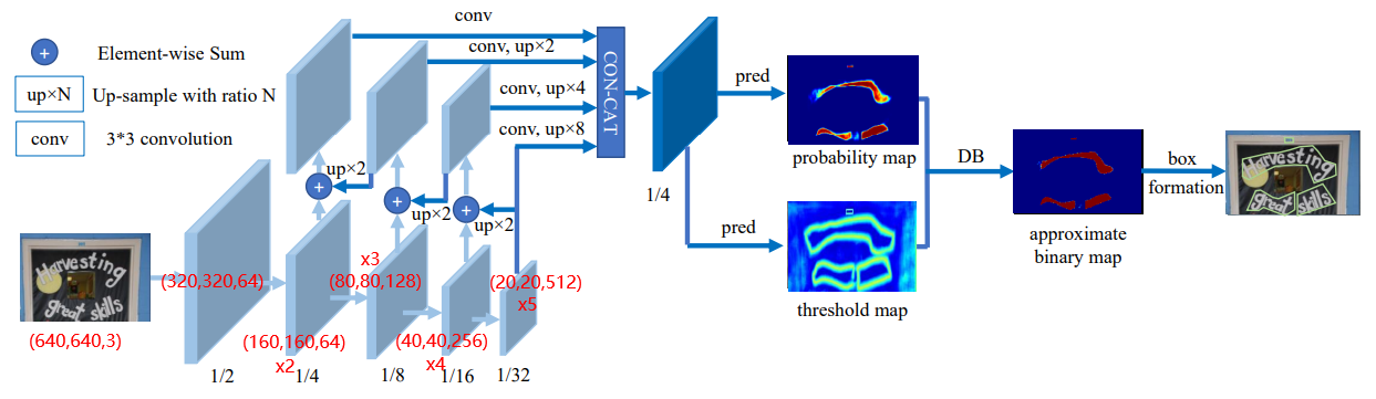
        # 以下是模拟的输入一张shape为(1,3,640,640)的图片的输出结果
        x = self.conv1(x)   	# 1,4,320,320
        x = self.bn1(x)
        x = self.relu(x)
        x = self.maxpool(x)     # 1,64,160,160

        x2 = self.layer1(x)     # 1,64,160,160
        x3 = self.layer2(x2)    # 1,128,80,80
        x4 = self.layer3(x3)    # 1,256,40,40
        x5 = self.layer4(x4)    # 1,512,20,20

        return x2, x3, x4, x5

还原到图中，如下所示：

3.1.5. 跳转到BasicBlock类

class BasicBlock(nn.Module):
    expansion = 1

    def __init__(self, inplanes, planes, stride=1, downsample=None, dcn=None):
        super(BasicBlock, self).__init__()
        self.with_dcn = dcn is not None
        self.conv1 = conv3x3(inplanes, planes, stride)      # 3*3卷积
        self.bn1 = BatchNorm2d(planes)                      # BN
        self.relu = nn.ReLU(inplace=True)                   # 激活
        self.with_modulated_dcn = False
        if not self.with_dcn:
            self.conv2 = nn.Conv2d(planes, planes, kernel_size=3, padding=1, bias=False)
        else:
            from torchvision.ops import DeformConv2d
            deformable_groups = dcn.get('deformable_groups', 1)
            # 3*3*2=18  每个前8个位置是x的偏移量，后8个位置是y的偏移量，偏移量是通过卷积学习出来的
            offset_channels = 18
            # 先通过卷积操作学出18个偏移值
            self.conv2_offset = nn.Conv2d(planes, deformable_groups * offset_channels, kernel_size=3, padding=1)
            # 可变形卷积
            # 再将学出来的18个偏移值传入DeformConv2d，进行可变形卷积
            self.conv2 = DeformConv2d(planes, planes, kernel_size=3, padding=1, bias=False)     
        self.bn2 = BatchNorm2d(planes)
        self.downsample = downsample
        self.stride = stride

    def forward(self, x):
        residual = x

        out = self.conv1(x)
        out = self.bn1(out)
        out = self.relu(out)

        # out = self.conv2(out)
        if not self.with_dcn:
            out = self.conv2(out)
        else:
            offset = self.conv2_offset(out)
            out = self.conv2(out, offset)
        out = self.bn2(out)

        if self.downsample is not None:
            residual = self.downsample(x)

        out += residual
        out = self.relu(out)

        return out

3.2. neck

特征提取网络：FPN
核心代码：self.neck = build_neck(neck_type, in_channels=self.backbone.out_channels, **model_config.neck)

3.2.1. 进入model.py

class Model(nn.Module):
    def __init__(self, model_config: dict):
        """
        PANnet
        :param model_config: 模型配置
        """
        super().__init__()
        model_config = Dict(model_config)
        backbone_type = model_config.backbone.pop('type')
        neck_type = model_config.neck.pop('type')
        head_type = model_config.head.pop('type')
        # 构建backbone网络
        self.backbone = build_backbone(backbone_type, **model_config.backbone)
        # 构建neck网络
        self.neck = build_neck(neck_type, in_channels=self.backbone.out_channels, **model_config.neck)
        # 构建head网络
        self.head = build_head(head_type, in_channels=self.neck.out_channels, **model_config.head)
        self.name = f'{backbone_type}_{neck_type}_{head_type}'

    def forward(self, x):
        _, _, H, W = x.size()
        backbone_out = self.backbone(x) 	# backbone_out = (p2, p3, p4, p5)
        neck_out = self.neck(backbone_out)  # neck_out shape(1, 256, 160, 160) 测试单张图片
        y = self.head(neck_out)
        y = F.interpolate(y, size=(H, W), mode='bilinear', align_corners=True)
        return y

3.2.2. 进入build_neck()方法

def build_neck(neck_name, **kwargs):
    assert neck_name in support_neck, f'all support neck is {support_neck}'
    neck = eval(neck_name)(**kwargs)
    return neck

3.2.3. 跳转到FPN.py中的init方法

class FPN(nn.Module):
    def __init__(self, in_channels, inner_channels=256, **kwargs):
        """
        :param in_channels: 基础网络输出的维度
        :param kwargs:
        """
        super().__init__()
        inplace = True
        self.conv_out = inner_channels      	# 输出channel  256
        inner_channels = inner_channels // 4    # 64
        # reduce layers
        # 输入是64个channel，输出是64个channel
        self.reduce_conv_c2 = ConvBnRelu(in_channels[0], inner_channels, kernel_size=1, inplace=inplace)
        # 输入是128个channel，输出是64个channel
        self.reduce_conv_c3 = ConvBnRelu(in_channels[1], inner_channels, kernel_size=1, inplace=inplace)
        # 输入是256个channel，输出是64个channel
        self.reduce_conv_c4 = ConvBnRelu(in_channels[2], inner_channels, kernel_size=1, inplace=inplace)
        # 输入是512个channel，输出是64个channel
        self.reduce_conv_c5 = ConvBnRelu(in_channels[3], inner_channels, kernel_size=1, inplace=inplace)
        # Smooth layers
        self.smooth_p4 = ConvBnRelu(inner_channels, inner_channels, kernel_size=3, padding=1, inplace=inplace)
        self.smooth_p3 = ConvBnRelu(inner_channels, inner_channels, kernel_size=3, padding=1, inplace=inplace)
        self.smooth_p2 = ConvBnRelu(inner_channels, inner_channels, kernel_size=3, padding=1, inplace=inplace)

        self.conv = nn.Sequential(
            nn.Conv2d(self.conv_out, self.conv_out, kernel_size=3, padding=1, stride=1),
            nn.BatchNorm2d(self.conv_out),
            nn.ReLU(inplace=inplace)
        )
        self.out_channels = self.conv_out

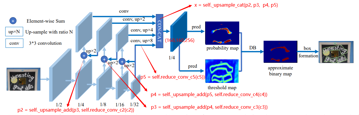
    def forward(self, x):
        c2, c3, c4, c5 = x
        # Top-down
        p5 = self.reduce_conv_c5(c5)
        p4 = self._upsample_add(p5, self.reduce_conv_c4(c4))
        p4 = self.smooth_p4(p4)
        p3 = self._upsample_add(p4, self.reduce_conv_c3(c3))
        p3 = self.smooth_p3(p3)
        p2 = self._upsample_add(p3, self.reduce_conv_c2(c2))
        p2 = self.smooth_p2(p2)

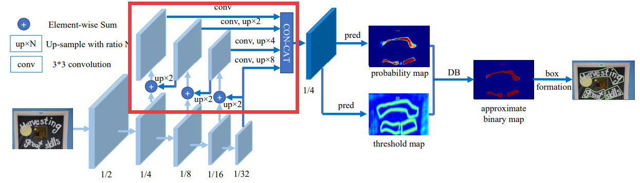
        x = self._upsample_cat(p2, p3, p4, p5)  # 拼接之后的维度  1,256,160,160  测试单张图片
        x = self.conv(x)
        return x

    def _upsample_add(self, x, y):
        return F.interpolate(x, size=y.size()[2:]) + y

    def _upsample_cat(self, p2, p3, p4, p5):
        h, w = p2.size()[2:]
        p3 = F.interpolate(p3, size=(h, w))
        p4 = F.interpolate(p4, size=(h, w))
        p5 = F.interpolate(p5, size=(h, w))
        return torch.cat([p2, p3, p4, p5], dim=1)

其中，_upsample_add方法和_upsample_cat方法还原到图中如下所示：

3.3. head

预测网络：CNN
核心代码：self.head = build_head(head_type, in_channels=self.neck.out_channels, **model_config.head)
在训练的时候需要预测出shrink_maps, threshold_maps, binary_maps

3.3.1. 进入model.py

class Model(nn.Module):
    def __init__(self, model_config: dict):
        """
        PANnet
        :param model_config: 模型配置
        """
        super().__init__()
        model_config = Dict(model_config)
        backbone_type = model_config.backbone.pop('type')
        neck_type = model_config.neck.pop('type')
        head_type = model_config.head.pop('type')
        # 构建backbone网络
        self.backbone = build_backbone(backbone_type, **model_config.backbone)
        # 构建neck网络
        self.neck = build_neck(neck_type, in_channels=self.backbone.out_channels, **model_config.neck)
        # 构建head网络
        self.head = build_head(head_type, in_channels=self.neck.out_channels, **model_config.head)
        self.name = f'{backbone_type}_{neck_type}_{head_type}'

    def forward(self, x):
        _, _, H, W = x.size()
        backbone_out = self.backbone(x) 	# backbone_out = (p2, p3, p4, p5)
        neck_out = self.neck(backbone_out)  # neck_out shape(1, 256, 160, 160) 测试单张图片
        y = self.head(neck_out)
        y = F.interpolate(y, size=(H, W), mode='bilinear', align_corners=True)
        return y

3.3.2. 进入build_head()方法

def build_head(head_name, **kwargs):
    assert head_name in support_head, f'all support head is {support_head}'
    head = eval(head_name)(**kwargs)
    return head

3.3.3. 跳转到DBHead.py中的DBHead类的init方法

class DBHead(nn.Module):
    def __init__(self, in_channels, out_channels, k=50):
        super().__init__()
        self.k = k
        self.binarize = nn.Sequential(
            nn.Conv2d(in_channels, in_channels // 4, 3, padding=1),
            nn.BatchNorm2d(in_channels // 4),
            nn.ReLU(inplace=True),
            nn.ConvTranspose2d(in_channels // 4, in_channels // 4, 2, 2),
            nn.BatchNorm2d(in_channels // 4),
            nn.ReLU(inplace=True),
            nn.ConvTranspose2d(in_channels // 4, 1, 2, 2),
            nn.Sigmoid())
        # 初始化二值图的权重参数
        self.binarize.apply(self.weights_init)
        # 初始化阈值图的权重参数
        self.thresh = self._init_thresh(in_channels)
        self.thresh.apply(self.weights_init)
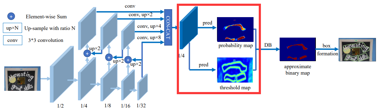
    def forward(self, x):
        # 预测shrink_maps
        shrink_maps = self.binarize(x)  # (1,1,640,640)
        # 预测threshold_maps
        threshold_maps = self.thresh(x) # (1,1,640,640)
        if self.training:
            # 预测binary_maps
            binary_maps = self.step_function(shrink_maps, threshold_maps)   	# (1,1,640,640)
            y = torch.cat((shrink_maps, threshold_maps, binary_maps), dim=1) 	# (1,3,640,640)
        else:
            y = torch.cat((shrink_maps, threshold_maps), dim=1)					# (1,2,640,640)
        return y
    ......

上面代码中，

shrink_maps = self.binarize(x)  # (1,1,640,640)

通过定义好的CNN来预测概率图

threshold_maps = self.thresh(x) # (1,1,640,640)

通过定义好的CNN来预测阈值图

binary_maps = self.step_function(shrink_maps, threshold_maps)   	# (1,1,640,640)

根据论文中定义好的公式来计算阈值图，其公式如下：

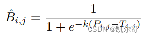
公式的实现代码如下：

def step_function(self, x, y):
    return torch.reciprocal(1 + torch.exp(-self.k * (x - y)))

3.4. 损失函数

3.4.1. 进入DB_loss.py

class DBLoss(nn.Module):
    def __init__(self, alpha=1.0, beta=10, ohem_ratio=3, reduction='mean', eps=1e-6):
        """
        Implement PSE Loss.
        :param alpha: binary_map loss 前面的系数
        :param beta: threshold_map loss 前面的系数
        :param ohem_ratio: OHEM的比例
        :param reduction: 'mean' or 'sum'对 batch里的loss 算均值或求和
        """
        super().__init__()
        assert reduction in ['mean', 'sum'], " reduction must in ['mean','sum']"
        self.alpha = alpha
        self.beta = beta
        # 交叉熵损失
        self.bce_loss = BalanceCrossEntropyLoss(negative_ratio=ohem_ratio)
        # 常用与分割任务中的dice loss
        self.dice_loss = DiceLoss(eps=eps)
        # l1 loss
        self.l1_loss = MaskL1Loss(eps=eps)
        self.ohem_ratio = ohem_ratio
        self.reduction = reduction

    def forward(self, pred, batch):
        # 以batchsize为1为例，pred的shape为(1,3,640,640)
        # batch 是一个字典，里面包含了img,threshold_mask,threshold_mask,thrink_map,thrink_mask 五个key
        shrink_maps = pred[:, 0, :, :]		# (1,640,640)
        threshold_maps = pred[:, 1, :, :]	# (1,640,640)
        binary_maps = pred[:, 2, :, :]		# (1,640,640)
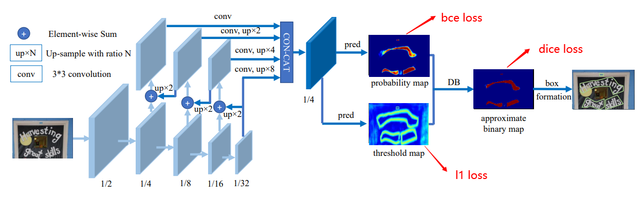
		# probability map 损失
        loss_shrink_maps = self.bce_loss(shrink_maps, batch['shrink_map'], batch['shrink_mask'])
        # threshold map 损失
        loss_threshold_maps = self.l1_loss(threshold_maps, batch['threshold_map'], batch['threshold_mask'])
        metrics = dict(loss_shrink_maps=loss_shrink_maps, loss_threshold_maps=loss_threshold_maps)
        if pred.size()[1] > 2:
            # approximate binary map 损失
            loss_binary_maps = self.dice_loss(binary_maps, batch['shrink_map'], batch['shrink_mask'])
            metrics['loss_binary_maps'] = loss_binary_maps
            loss_all = self.alpha * loss_shrink_maps + self.beta * loss_threshold_maps + loss_binary_maps
            metrics['loss'] = loss_all
        else:
            metrics['loss'] = loss_shrink_maps
        return metrics

上面代码中，

pred

shape：(1,3,640,640)

- 1表示batchsize为1；
- 3分别表示shrink_maps，threshold_maps，binary_maps的预测结果；
- 后面两个维度分别表示图片的h和w。

batch

img：shape为(1,3,640,640)，经过预处理之后的图片
threshold_map(gt)：shape为(1,640,640)，经过标注之后的阈值图，可视化结果如下图所示

threshold_mask：shape为(1,640,640)，可视化结果如下图所示

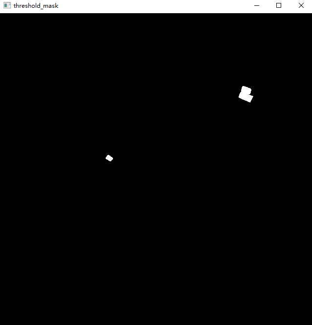
除文本区域是白色以外，其他区域都是黑色。

shrink_map(gt)：shape为(1,640,640)，经过标注之后的概率图，即缩放之后的文本框。可视化结果如下图所示

shrink_mask：shape为(1,640,640)，黑色部分表示图片中不需要关注(面积小的或者不需要识别的)的那些文本框，需要注意的是，shrink_mask上的黑色框为原始的文本框，即未经过shrink的框。可视化结果如下图所示

shrink_maps：预测出的概率图，其shape为(1,640,640)

threshold_maps：预测出的阈值图，其shape为(1,640,640)

binary_maps：预测出的二值图，其shape为(1,640,640)

3.4.2. BCELoss

走到下面这行代码，

loss_shrink_maps = self.bce_loss(shrink_maps, batch['shrink_map'], batch['shrink_mask'])

然后跳转到BalanceCrossEntropyLoss类，执行forward方法，计算loss

def forward(self,
			pred: torch.Tensor,
			gt: torch.Tensor,
			mask: torch.Tensor,
			return_origin=False):
	positive = (gt * mask).byte()       # 得到的是我们所关注的那些文本框，即正例
	negative = ((1 - gt) * mask).byte()	# 除开这些文本框之外的其他图片区域，即负例
	positive_count = int(positive.float().sum())	# 计算正例的个数
    # 计算负例的个数，这里对附录设置了限制，最多为正例的3倍。self.negative_ratio=3
	negative_count = min(int(negative.float().sum()), int(positive_count * self.negative_ratio))
	# 计算交叉熵损失
    loss = nn.functional.binary_cross_entropy(pred, gt, reduction='none')
	positive_loss = loss * positive.float()     # 正例的loss
	negative_loss = loss * negative.float()     # 负例的loss
	# negative_loss, _ = torch.topk(negative_loss.view(-1).contiguous(), negative_count)
	negative_loss, _ = negative_loss.view(-1).topk(negative_count)
	# 分母加上self.eps，防止出现分母为零的情况
	balance_loss = (positive_loss.sum() + negative_loss.sum()) / (positive_count + negative_count + self.eps)
	if return_origin:
		return balance_loss, loss
	return balance_loss

BCELoss 示例

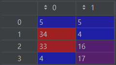
BCELoss 的计算方式：对输出向量的每个元素单独使用交叉熵损失函数，然后计算平均值。

# 预测值
output = torch.randn(3, 3)

# 激活函数
active_func = nn.Sigmoid()
output = active_func(output)
print(output)

# 标签值
target = torch.FloatTensor([[0, 1, 1], [1, 1, 1], [0, 0, 0]])
loss = nn.BCELoss()

loss = loss(output, target)
print(loss)


tensor([[0.3194, 0.4580, 0.2615],
        [0.6796, 0.5903, 0.5908],
        [0.4377, 0.4028, 0.4199]])

tensor(0.6203)

3.4.3. MaskL1Loss

走到下面这行代码，

loss_threshold_maps = self.l1_loss(threshold_maps, batch['threshold_map'], batch['threshold_mask'])

然后跳转到MaskL1Loss类，执行forward方法，计算loss

class MaskL1Loss(nn.Module):
    def __init__(self, eps=1e-6):
        super(MaskL1Loss, self).__init__()
        self.eps = eps

    def forward(self, pred: torch.Tensor, gt, mask):
        # pred 预测值
        # gt 标签值
        # mask 需要过滤的区域
        loss = (torch.abs(pred - gt) * mask).sum() / (mask.sum() + self.eps)        # 只计算需要关注的文本框的损失
        return loss

L1Loss 实例

L1Loss 的计算方式：平均绝对误差

import torch.nn as nn
import torch

pixelwise_loss = nn.L1Loss(reduction='mean')  # 平均绝对误差,L1-损失

x1 = torch.tensor([[1, 1], [1, 1]])
x2 = torch.tensor([[0.125, 0.5], [0.5, 0.5]])
y = pixelwise_loss(x2, x1)
print('L1Loss:', y.item())
print(((1 - 0.125) + (1 - 0.5) + (1 - 0.5) + (1 - 0.5)) / 4)



L1Loss: 0.59375
0.59375

3.4.4. DiceLoss

走到下面这行代码，

loss_binary_maps = self.dice_loss(binary_maps, batch['shrink_map'], batch['shrink_mask'])

然后跳转到DiceLoss类，执行forward方法，计算loss

class DiceLoss(nn.Module):
    '''
    Loss function from https://arxiv.org/abs/1707.03237,
    where iou computation is introduced heatmap manner to measure the
    diversity bwtween tow heatmaps.
    '''

    def __init__(self, eps=1e-6):
        super(DiceLoss, self).__init__()
        self.eps = eps

    def forward(self, pred: torch.Tensor, gt, mask, weights=None):
        '''
        pred: one or two heatmaps of shape (N, 1, H, W),
            the losses of tow heatmaps are added together.
        gt: (N, 1, H, W)
        mask: (N, H, W)
        '''
        return self._compute(pred, gt, mask, weights)

    def _compute(self, pred, gt, mask, weights):
        if pred.dim() == 4:
            pred = pred[:, 0, :, :]
            gt = gt[:, 0, :, :]
        assert pred.shape == gt.shape
        assert pred.shape == mask.shape
        if weights is not None:
            assert weights.shape == mask.shape
            mask = weights * mask
        intersection = (pred * gt * mask).sum()
        union = (pred * mask).sum() + (gt * mask).sum() + self.eps
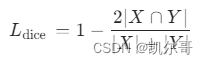
        loss = 1 - 2.0 * intersection / union
        assert loss <= 1
        return loss

其中，DiceLoss的数学计算公式如下所示：