代码分享 | EEG数据的等效偶极子源定位

文章来源于微信公众号（茗创科技），欢迎有兴趣的朋友搜索关注。

关于偶极子源定位：是指在 64~128 多导头皮脑电图记录的基础上，运用计算机数学模型推算自发或诱发脑电活动的起源，可用于癫痫外科术前辅助棘波起源的定位或诱发电位起源的研究。

如何用 DIPFIT 拟合一个偶极子与 EEG 或 ERP 的头皮图？

EEGLAB 有一个命令行函数可以允许 DIPFIT 进行拟合。拟合只能在选定的时间点进行，而不能在整个时间窗口中进行。在平均 ERP 波形中拟合 100ms 的时间点，可以使用以下 MATLAB 命令。
 

eeglab; close; % add path
eeglabp = fileparts(which('eeglab.m'));
EEG = pop_loadset(fullfile(eeglabp, 'sample_data', 'eeglab_data_epochs_ica.set'));

% Find the 100-ms latency data frame
latency = 0.100;
pt100 = round((latency-EEG.xmin)*EEG.srate);

% Find the best-fitting dipole for the ERP scalp map at this timepoint
erp = mean(EEG.data(:,:,:), 3);
dipfitdefs;

% Use MNI BEM model
EEG = pop_dipfit_settings( EEG, 'hdmfile',template_models(2).hdmfile,'coordformat',template_models(2).coordformat,...
    'mrifile',template_models(2).mrifile,'chanfile',template_models(2).chanfile,...
    'coord_transform',[0.83215 -15.6287 2.4114 0.081214 0.00093739 -1.5732 1.1742 1.0601 1.1485] ,'chansel',[1:32] );
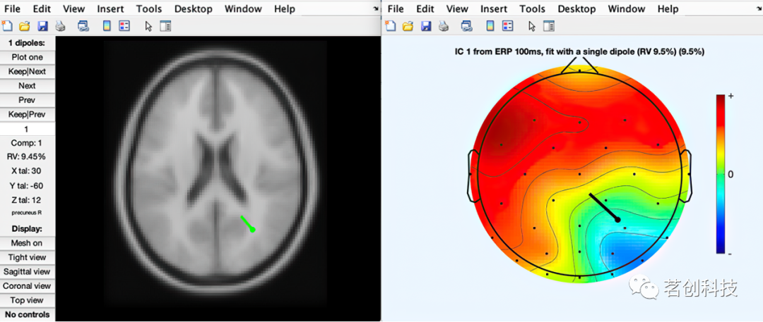
[ dipole, model, TMPEEG] = dipfit_erpeeg(erp(:,pt100), EEG.chanlocs, 'settings', EEG.dipfit, 'threshold', 100);

% plot the dipole in 3-D
pop_dipplot(TMPEEG, 1, 'normlen', 'on');

% Plot the dipole plus the scalp map
figure; pop_topoplot(TMPEEG,0,1, [ 'ERP 100ms, fit with a single dipole (RV ' num2str(dipole(1).rv*100,2) '%)'], 0, 1);

运行脚本后会生成这样两张图。

注：使用 eLoreta 也可以定位 EEG/ERP 源。

使用 DIPFIT/Fieldtrip 进行高级源重构。

DIPFIT 依赖于 Fieldtrip。开发者对 DIPFIT 进行了重新设计，使其能够使用 Fieldtrip 函数。以下是关于如何使用应用于 EEGLAB 数据集中的 Fieldtrip 执行源建模的简短教程。

先使用 DIPFIT 将电极位置与所选择的头部模型(菜单项工具→使用 DIPFIT 定位偶极子→头部模型和设置)对齐。得到的 DIPFIT 信息可以用来在 Fieldtrip 中执行源定位。

对体素进行源重构。

下面的第一个代码片段为 3-D 网格生成引导场矩阵(和 eLoreta 一起使用)。

%% First load a dataset in EEGLAB.
% Then use EEGLAB menu item <em>Tools > Locate dipoles using DIPFIT > Head model and settings</em>
% to align electrode locations to a head model of choice
% The eeglab/fieldtrip code is shown below:

eeglab                        % start eeglab
eeglabPath = fileparts(which('eeglab'));                 % save its location
bemPath = fullfile(eeglabPath, 'plugins', 'dipfit', 'standard_BEM');    % load the dipfit plugin
EEG = pop_loadset(fullfile(eeglabPath, 'sample_data', 'eeglab_data_epochs_ica.set'));   % load the sample eeglab epoched dataset
EEG = pop_dipfit_settings( EEG, 'hdmfile',fullfile(bemPath, 'standard_vol.mat'), ...
           'coordformat','MNI','mrifile',fullfile(bemPath, 'standard_mri.mat'), ...
           'chanfile',fullfile(bemPath, 'elec', 'standard_1005.elc'), ...
           'coord_transform',[0.83215 -15.6287 2.4114 0.081214 0.00093739 -1.5732 1.1742 1.0601 1.1485] , ...

然后使用 Fieldtrip 的 ft_prepare_leadfield 函数计算引导场矩阵。注意，头部模型也可以用于评估体素是在大脑内部还是外部。

%% Leadfield Matrix calculation
dataPre = eeglab2fieldtrip(EEG, 'preprocessing', 'dipfit');   % convert the EEG data structure to fieldtrip

cfg = [];
cfg.channel = {'all', '-EOG1'};
cfg.reref = 'yes';
cfg.refchannel = {'all', '-EOG1'};
dataPre = ft_preprocessing(cfg, dataPre);

vol = load('-mat', EEG.dipfit.hdmfile);

cfg            = [];
cfg.elec       = dataPre.elec;
cfg.headmodel  = vol.vol;
cfg.resolution = 10;   % use a 3-D grid with a 1 cm resolution
cfg.unit       = 'mm';
cfg.channel    = { 'all' };
[sourcemodel] = ft_prepare_leadfield(cfg);

使用现在生成的引导场矩阵进行源重构。这里，使用 eLoreta 为 ERP 的假定来源建模。这一步，可以用其他方法来代替 eLoreta，比如相干源的动态成像“dics”（感兴趣的小伙伴可以在 Fieldtrip 上了解关于这步的更多信息，网址为：https://www.fieldtriptoolbox.org/tutorial/beamformer/）。

%% Compute an ERP in Fieldtrip. Note that the covariance matrix needs to be calculated here for use in source estimation.
cfg                  = [];
cfg.covariance       = 'yes';
cfg.covariancewindow = [EEG.xmin 0]; % calculate the average of the covariance matrices
                                   % for each trial (but using the pre-event baseline  data only)
dataAvg = ft_timelockanalysis(cfg, dataPre);

% source reconstruction
cfg             = [];
cfg.method      = 'eloreta';
cfg.sourcemodel = sourcemodel;
cfg.headmodel   = vol.vol;
source          = ft_sourceanalysis(cfg, dataAvg);  % compute the source model

使用 Fieldtrip 函数进行绘制，画出不同偶极子的方向轴。

%% Plot Loreta solution
cfg = [];
cfg.projectmom = 'yes';
cfg.flipori = 'yes';
sourceProj = ft_sourcedescriptives(cfg, source);

cfg = [];
cfg.parameter = 'mom';
cfg.operation = 'abs';
sourceProj = ft_math(cfg, sourceProj);

cfg              = [];
cfg.method       = 'ortho';
cfg.funparameter = 'mom';
figure; ft_sourceplot(cfg, sourceProj);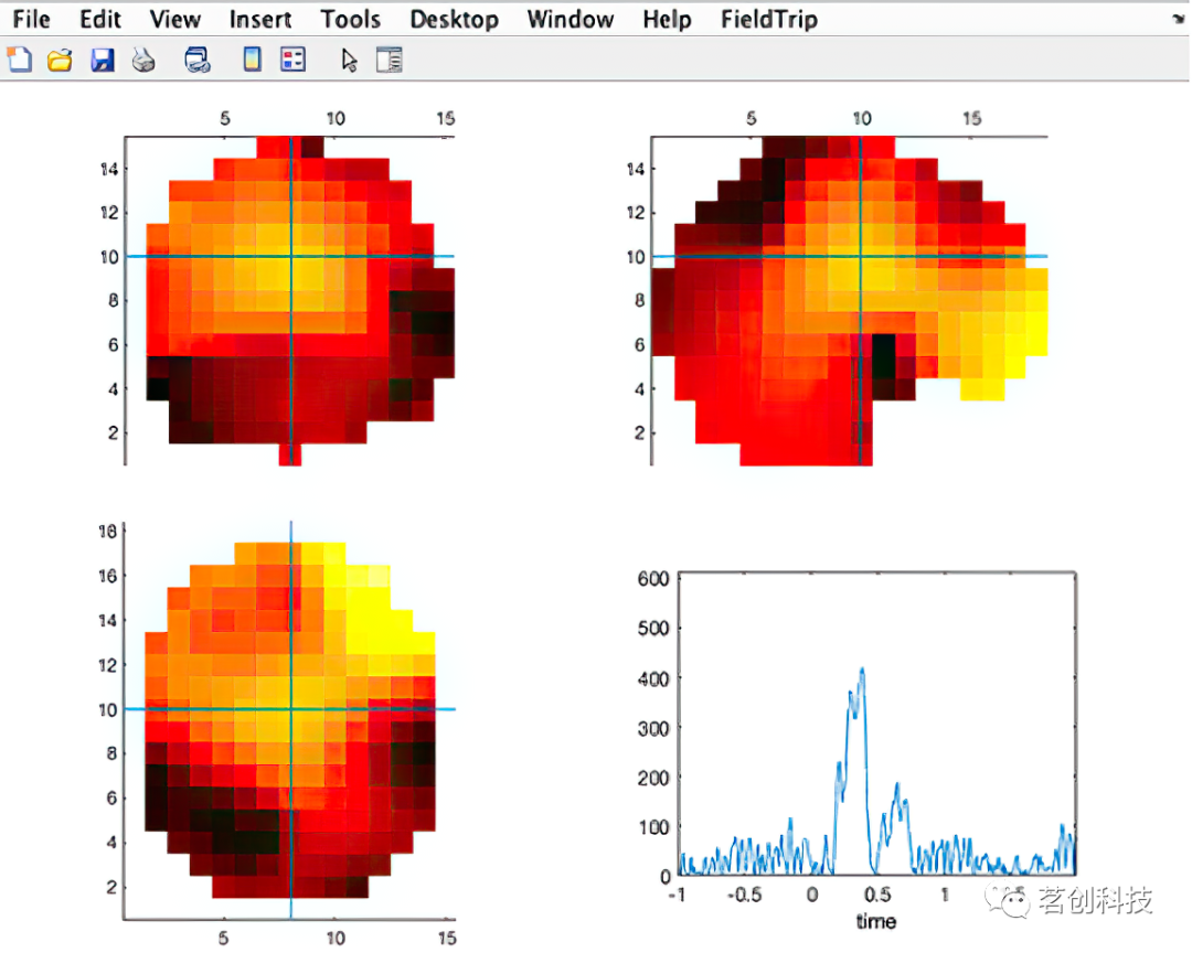

选择感兴趣的潜伏期，就可以将其投射到高分辨率 MRI 中(head image)。下面显示了头模的核磁共振切片的全脑功率。

%% project sources on MRI and plot solution
mri = load('-mat', EEG.dipfit.mrifile);
mri = ft_volumereslice([], mri.mri);

cfg              = [];
cfg.downsample   = 2;
cfg.parameter    = 'pow';
source.oridimord = 'pos';
source.momdimord = 'pos';
sourceInt  = ft_sourceinterpolate(cfg, source , mri);

cfg              = [];
cfg.method       = 'slice';
cfg.funparameter = 'pow';
ft_sourceplot(cfg, sourceInt);

在头皮表面进行源重构。

或者，用下面的代码在 MNI 空间中生成一个真实的 3-D 网格的引导场矩阵。这里，需要在 DIPFIT 设置菜单中选择头部模型时选择 MNI BEM 头部模型。不同的网格版本可以使用不同的分辨率（有关更多信息，请查看网址：https://www.fieldtriptoolbox.org/template/sourcemodel/）。

%% Prepare leadfield surface
[ftVer, ftPath] = ft_version;
sourcemodel = ft_read_headshape(fullfile(ftPath, 'template', 'sourcemodel', 'cortex_8196.surf.gii'));

cfg           = [];
cfg.grid      = sourcemodel;    % source points
cfg.headmodel = vol.vol;        % volume conduction model
leadfield = ft_prepare_leadfield(cfg, dataAvg);

前一节中的代码使用了 eLoreta，本节将使用最小范数估计(MNE)。MNE 和 eLoreta 都可以在每个延迟时间执行源重构(假设使用 EEG 时间序列作为输入)。

%% Surface source analysis
cfg               = [];
cfg.method        = 'mne';
cfg.grid          = leadfield;
cfg.headmodel     = vol.vol;
cfg.mne.lambda    = 3;
cfg.mne.scalesourcecov = 'yes';
source            = ft_sourceanalysis(cfg, dataAvg);

现在绘制全脑功率，使用相同的方法，可以创建 MNE 源解决方法随时间变化的图片展示。

%% Surface source plot
cfg = [];
cfg.funparameter = 'pow';
cfg.maskparameter = 'pow';
cfg.method = 'surface';
cfg.latency = 0.4;
cfg.opacitylim = [0 200];
ft_sourceplot(cfg, source);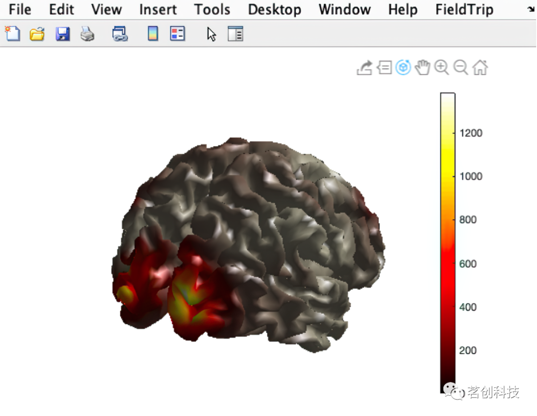

也可以通过在上面的图像上叠加 BEM 网格来查看源模型网格与 BEM 头部模型网格的对齐情况，如下图所示。

hold on; ft_plot_mesh(vol.vol.bnd(3), 'facecolor', 'red', 'facealpha', 0.05, 'edgecolor', 'none');
hold on; ft_plot_mesh(vol.vol.bnd(2), 'facecolor', 'red', 'facealpha', 0.05, 'edgecolor', 'none');
hold on; ft_plot_mesh(vol.vol.bnd(1), 'facecolor', 'red', 'facealpha', 0.05, 'edgecolor', 'none');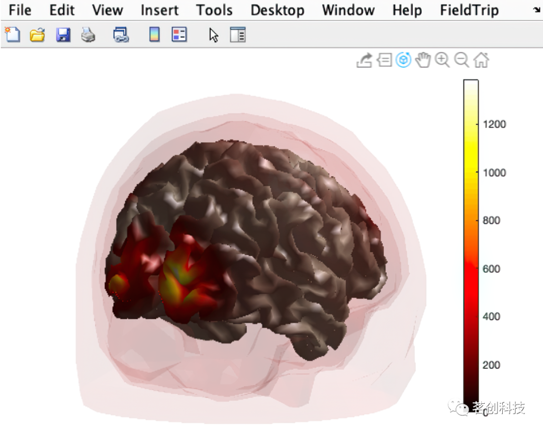

参考来源：

https://github.com/sccn/sccn.github.io/blob/master/tutorials/09_source/EEG_sources.md

https://www.fieldtriptoolbox.org/tutorial/beamformer/

https://www.fieldtriptoolbox.org/template/sourcemodel/