Backpropagation, Intuitions

原文地址：http://cs231n.github.io/optimization-2/

################################################################

内容列表：

１．介绍

２．简单表达式，解释梯度

３．复合表达式，链式法则，反向传播

４．反向传播的直观理解

５．模块化：Sigmoid案例

６．实际应用反向传播：分段计算

７．逆向流模式（Patterns in backward flow）

８．向量运算的梯度（Gradients for vectorized operations）

９．总结

#########################################################################3

Introduction

Motivation. 本节中，我们将对反向传播（backpropagation）有一个直观的认识，其是通过对链式法则（chain rule）的递归应用来计算表达式的梯度。理解这个过程以及它的微妙之处，这对于你有效地开发，设计和调试神经网络有关键的影响。

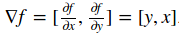
Problem statement. 本节的核心问题如下：我们得到一些函数，其中参数是一组输入参数，我们需要计算函数在输入向量处的梯度（i.e.）。

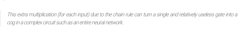
Motivation. 回忆我们对这个问题感兴趣的最主要原因，是因为在神经网络的特定例子中，对应于损失函数（），然后输入由训练数据和神经网络权重组成。举个例子，损失为SVM损失函数，输入为训练数据和权重以及偏置。注意（机器学习中通常是这样的）假定训练数据是固定的，我们可以控制权重的设定。因此，尽管我可可以使用反向传播来计算输入样本的梯度，但实际上通常仅计算参数的梯度（e.g.），所以我们可以使用反向传播来进行参数更新。然而，我们在本节课后面将会看到，在上的梯度有时也是有用的，举个例子，为了可视化和解释神经网络能做什么的情况。

如果你对于使用链式法则推导梯度很熟悉，我们仍然希望你能够浏览一遍，因为本文展示了一个很少学习的观点，即把反向传播作为真实电路图中的逆向电流，你可能从中会有收获。

Simple expressions and interpretation of the gradient

让我们以一个简单的表达式开始，这样是为了以后更复杂的表达式开发符号和约定。考虑一个简单的两个数字相乘的函数：。推导每一个输入的偏导数是一个简单的微积分问题：

Interpretation. 记住：导数表示一个函数在某个点上，在有限小的区间内，变量改变，导致函数改变的速率（Keep in mind what the derivatives tell you: They indicate the rate of change of a function with respect to that variable surrounding an infinitesimally small region near a particular point）:

技术说明：左侧的除号并不像右侧的除号，并不是一个除法操作。相反，这个符号表明操作符被应用到函数上，然后返回一个不同的函数（导数）。一个很好理解的方式，当参数很小时，函数可以通过一条直线来近似代替，而导数就是它的斜率。换句话说，每一个变量上的导数告诉你整个表达式在这个值上的敏感性（the derivative on each variable tells you the sensitivity of the whole expression on its value）。举个例子，如果，那么函数值，在指定上的导数为。这告诉我们，如果我们想要小小的增加变量的值，那么对于表达式的影响就是函数值减小（由于导数有负的符号），并且3倍于增加的变量值。通过重新排列上面的等式可以看出：。相类似的，如果增加变量的值，增加量为很小的值，那么函数输出将会增加（因为导数有正的符号），并且增加量为。

如前所述，导数是偏导数的向量集合：。通常为了简便，我们都用术语来代替正确说法。

我们也可以为加法运算推导导数：

如上所述，无论变量如何改变，其导数都是1。这是有道理的，因为无论是增加还是的值都会增加函数的输出，并且增加的速率独立于的值（并不像之前的乘法所示）。本节将要提到的最后一个函数是max操作：

如上所示，如果x>=y，那么x的梯度为1，y的梯度为0；反之，y的梯度为1，而x的梯度为0。直观上讲，如果输入是，那么最大值是4，那么函数对于变量y不敏感。也就是说，如果我们用极小值h增加y，函数值还是4，所以梯度为0。当然，如果给y加上一个很大的值（e.g. 比2更大），那么函数f的输出必然改变，but the derivatives tell us nothing about the effect of such large changes on the inputs of a function; They are only informative for tiny, infinitesimally small changes on the inputs, as indicated by the in its definition.

Compound expressions with chain rule

现在开始更复杂的表达式：由多个功能函数组成，比如。虽然表达式还是足够简单的，可以直接求导，但在这里我们要用一个特殊的方法来实现，这样有助于我们直观地理解反向传播。特别的，上述表达式可以分解为两个：。另外，如前所示，我们可以直接求出这两个子函数的导数。就是和的乘积，所以，并且是和的相加，所以。然而，我们不需要关心中间值的梯度－并没有用处。相反，我们应该计算出相对于变量的梯度。链式法则（thechain rule）告诉我们，同时“chain”这些梯度表达式的正确方式是通过乘法。举个例子，。实际上，这是一个简单的拥有两个输入参数的乘法函数，所以拥有两个梯度。代码如下：

# set some inputs
x = -2; y = 5; z = -4

# perform the forward pass
q = x + y # q becomes 3
f = q * z # f becomes -12

# perform the backward pass (backpropagation) in reverse order:
# first backprop through f = q * z
dfdz = q # df/dz = q, so gradient on z becomes 3
dfdq = z # df/dq = z, so gradient on q becomes -4
# now backprop through q = x + y
dfdx = 1.0 * dfdq # dq/dx = 1. And the multiplication here is the chain rule!
dfdy = 1.0 * dfdq # dq/dy = 1

最后，我们得到了梯度 ，which tell us the sensitivity of the variables   on  ！这个是反向传播的最简单的例子。下面，我们想要使用一个更加简洁的符号，so that we don’t have to keep writing the   part。That is, for example instead of  　we would simply write  ，and always assume that the gradient is with respect to the final output.

上述计算过程可以通过电路图展现：

Intuitive understainding of backpropagation

注意，反向传播是一个完美的局部操作。电路图中的每一个门得到一些输入后回马上计算两件事情：１．输出值；２．相对于输出值，它的输出的局部梯度。注意，做这些事情是完全独立的，并不需要考虑全局的任何细节（ Notice that the gates can do this completely independently without being aware of any of the details of the full circuit that they are embedded in.）。然而，一旦前向操作完成，在反向传播的时候，the gate will eventually learn about the gradient of its output value on the final output of the entire circuit。链式法则说明了 the gate should take that gradient and multiply it into every gradient it normally computes for all of its inputs.

举个例子来直观说明。加法门（the add gate）收到输入为[-2, 5]，计算得到3。因为这个门是加法操作，所以它的两个输入的局部梯度值都是1。和电路的其他部分操作得到最终的输出值-12。在反向传播时，链式法则被递归的应用在电路的逆流，加法门（也是乘法门的一个输入）学习到它的输出梯度是-4。假如我们人格化电路，想要得到更高的输出（这样可以帮助理解），那么我们可以想象电路“想要”加法门的输出能够变得更低（因为加法门的输出梯度为-4）。To continue the recurrence and to chain the gradient, 加法门得到梯度后将和输入的局部梯度相乘（使得x和y上的梯度变成）。注意这又一个好的影响：如果x,y将要减小（相对应于负的梯度值），那么加法门的输出也会减小，反过来使得乘法门的输出下降。

Backpropagation can thus be thought of as gates communicating to each other (through the gradient signal) whether they want their outputs to increase or decrease (and how strongly), so as to make the final output value higher.

Modularity：Sigmoid example

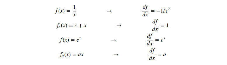
上面介绍的门是相对任意的。任何求导函数都可以作为一个门，我们也可以把多个门组成一个门，或者方便的话，也可以分解一个函数到多个门。下面是另一个表达式，可以证明这个观点：

我们将在本节后面看到，这个表达式描述了一个2维神经元（拥有输入和权重），使用的是sigmoid激活函数。不过现在仅仅简单的考虑为一个函数（输入w,x均为单个数值）。这个函数有多个门组成。 In addition to the ones described already above (add, mul, max), there are four more:

函数表示输入加上常量c，函数表示输入乘以常量a。这两个是加法和乘法操作的特殊例子，在这里我们介绍它们作为（新的）一元门，因为我们需要常数c和a的梯度。完整的电路图如下：

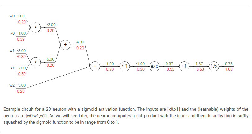
In the example above, we see a long chain of function applications that operates on the result of the dot product between w,x. 这些操作应用表示的函数称为sigmoid函数（the sigmoid function）。事实证明，the derivative of the sigmoid function with respect to its input simplifies if you perform the derivation (after a fun tricky part where we add and subtract a 1 in the numerator):

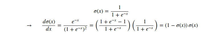
就像我们看到的，梯度简化了，变得非常简单。举个例子，sigmoid表达式得到输入1.0，计算得出0.73，那么此时的局部梯度（local gradient）就是，as the circuit computed before (see the image above)，except this way it would be done with a single, simple and efficient expression (and with less numerical issues)。因此在实际应用中，这是非常有用的，可以把这些操作组成一个门即可。代码如下：

w = [2,-3,-3] # assume some random weights and data
x = [-1, -2]

# forward pass
dot = w[0]*x[0] + w[1]*x[1] + w[2]
f = 1.0 / (1 + math.exp(-dot)) # sigmoid function

# backward pass through the neuron (backpropagation)
ddot = (1 - f) * f # gradient on dot variable, using the sigmoid gradient derivation
dx = [w[0] * ddot, w[1] * ddot] # backprop into x
dw = [x[0] * ddot, x[1] * ddot, 1.0 * ddot] # backprop into w
# we're done! we have the gradients on the inputs to the circuit

Implementation protip：staged backpropagation. 如上代码所示，这有助于分解前向过程为分段计算，这样更容易反向传播。举个例子，我们创造了一个中间变量 ，它表示 和 的点积操作结果。在反向传播过程中，我们成功的（以相反方向）计算了相应的变量（e.g. ，以及最终的 ）的梯度。

本节重点是弄清楚反向传播是如何计算的，以及为了方便起见，前向函数的哪些部分可以作为门。It helps to be aware of which parts of the expression have easy local gradients, so that they can be chained together with the least amount of code and effort.

Backprop in practice：Staged computation

下面是另外一个例子：

需要澄清的是，这个函数是完全没有用的，它仅仅是反向传播的一个很好的练习。需要强调的是，如果你想要对x或y求导数，那么应该以很大的或很复杂的表达式结束（ It is very important to stress that if you were to launch into performing the differentiation with respect to either x or y, you would end up with very large and complex expressions.）。然而，事实证明这是完全不需要的，because we don’t need to have an explicit function written down that evaluates the gradient。我们仅仅需要知道如何计算梯度。下面展示了我们如何构建the forward pass of such expression：

x = 3 # example values
y = -4

# forward pass
sigy = 1.0 / (1 + math.exp(-y)) # sigmoid in numerator   #(1)
num = x + sigy # numerator                               #(2)
sigx = 1.0 / (1 + math.exp(-x)) # sigmoid in denominator #(3)
xpy = x + y                                              #(4)
xpysqr = xpy**2                                          #(5)
den = sigx + xpysqr # denominator                        #(6)
invden = 1.0 / den                                       #(7)
f = num * invden # done!                                 #(8)

在上述过程结束后，我们就完成了前向过程的计算。注意，我们在代码中赋值了多个中间变量，每一个中间变量都仅有简单的表达式（我们以及知道这个表达式的局部梯度）。因此，计算反向过程是很容易的：我们将反向计算前向过程中出现的每一个变量（ ），在这些变量前面加上 表示梯度
。另外，在反向传播中，每一步都包括计算表达式的局部梯度，以及chaining it with the gradient on that expression with a multiplication。代码如下：

# backprop f = num * invden
dnum = invden # gradient on numerator                             #(8)
dinvden = num                                                     #(8)
# backprop invden = 1.0 / den 
dden = (-1.0 / (den**2)) * dinvden                                #(7)
# backprop den = sigx + xpysqr
dsigx = (1) * dden                                                #(6)
dxpysqr = (1) * dden                                              #(6)
# backprop xpysqr = xpy**2
dxpy = (2 * xpy) * dxpysqr                                        #(5)
# backprop xpy = x + y
dx = (1) * dxpy                                                   #(4)
dy = (1) * dxpy                                                   #(4)
# backprop sigx = 1.0 / (1 + math.exp(-x))
dx += ((1 - sigx) * sigx) * dsigx # Notice += !! See notes below  #(3)
# backprop num = x + sigy
dx += (1) * dnum                                                  #(2)
dsigy = (1) * dnum                                                #(2)
# backprop sigy = 1.0 / (1 + math.exp(-y))
dy += ((1 - sigy) * sigy) * dsigy                                 #(1)
# done! phew

注意以下几点：

Cache forward pass variables. 如果把前向过程的变量保存下来，这对于反向传播操作很有用处。In practice you want to structure your code so that you cache these variables, and so that they are available during backpropagation. If this is too difficult, it is possible (but wasteful) to recompute them.

Gradients add up at forks. 正向表达式多次使用变量，所以，当我们执行反向传播的时候，我们应该使用而不是来累积这些变量的梯度（或者我们可以重写）。 This follows the multivariable chain rule in Calculus, which states that if a variable branches out to different parts of the circuit, then the gradients that flow back to it will add。

Patterns in backward flow

反向流的梯度可以很直观地解释清楚。举个例子，神经网络上最常用的3个门（加法，乘法，max）都有很简单的解释（in terms of how they act during backpropagation）。考虑下面的电路图：

从上面的电路图中可以看出，

加法门（the add gate）得到输出的梯度后，会同样分配给它的输入，而不管输入在前向操作中的大小。这是因为加法操作的局部梯度是1.0，so the gradients on all inputs will exactly equal the gradients on the output because it will be multiplied by x1.0 (and remain unchanged)。In the example circuit above, note that the + gate routed the gradient of 2.00 to both of its inputs, equally and unchanged.

The max gate routes the gradient. Unlike the add gate which distributed the gradient unchanged to all its inputs, the max gate distributes the gradient (unchanged) to exactly one of its inputs (the input that had the highest value during the forward pass). This is because the local gradient for a max gate is 1.0 for the highest value, and 0.0 for all other values. In the example circuit above, the max operation routed the gradient of 2.00 to the z variable, which had a higher value than w, and the gradient on w remains zero.

The multiply gate is a little less easy to interpret. Its local gradients are the input values (except switched), and this is multiplied by the gradient on its output during the chain rule. In the example above, the gradient on x is -8.00, which is -4.00 x 2.00.

Unintuitive effects and their consequences. 注意，如果乘法门的一个输入值很小而另一个很大，then the multiply gate will do something slightly unintuitive：它会分配一个相对大的梯度值给小的输入值，而分配一个很小的梯度给大的输入。Note that in linear classifiers where the weights are dot producted   (multiplied) with the inputs, this implies that the scale of the data has an effect on the magnitude of the gradient for the weights. 举个例子，在预处理阶段，将所有的输入样本都乘上1000，那么权重的梯度也会增加1000倍，and you’d have to lower the learning rate by that factor to compensate。这也是为什么预处理很重要。And having intuitive understanding for how the gradients flow can help you debug some of these cases.

Gradients for vectorized operations

以上各部分均为单变量，下面将扩展为矩阵和向量操作。必须注意维度和转置操作。

Matrix-Matrix multiply gradient. 矩阵乘法可能是最复杂的操作（which generalizes all matrix-vector and vector-vector）:

# forward pass
W = np.random.randn(5, 10)
X = np.random.randn(10, 3)
D = W.dot(X)

# now suppose we had the gradient on D from above in the circuit
dD = np.random.randn(*D.shape) # same shape as D
dW = dD.dot(X.T) #.T gives the transpose of the matrix
dX = W.T.dot(dD)

提示：使用维度分析（dimension analysis）! 并不需要记住 和 的表达式，因为这些都可以很容易的基于维度被重新推导。For instance, we know that the gradient on the weights  must be of the same size as  after it is computed, and that it must depend on matrix multiplication of  and  (as is the case when both are single numbers and not matrices). There is always exactly one way of achieving this so that the dimensions work out. For example,  is of size [10 x 3] and  of size [5 x 3], so if we want  and  has shape [5 x 10], then the only way of achieving this is with , as shown above.

Work with small, explicit examples. 可能有些向量表达式不易直接推导出梯度。我们的建议是先写成一个最小的向量例子，推导出梯度，then generalize the pattern to its efficient, vectorized form

Summary

１）我们直观理解了梯度的含义，它们如何反向传播，它们如何相互联系以及如何使得最终输出更高

２）我们讨论了在实际应用中分段计算（staged computation）对于反向传播的重要性。你应该尽量把函数分解为各个模块（要求：在每个模块中你很容易就能推导出局部梯度），然后通过链式法则链接这些模块。最重要的是，你不要把这些表达式写在纸上进行演算，因为我们并不需要知道计算输入参数梯度的确切公式。因此，把复杂的表达式分为了多个简单的表达式，这样，就可以独立求导（the stages will be matrix vector multiplies, or max operations, or sum operations, etc.）并且进行反向传播运算。

下一节我们将开始定义神经网络，and backpropagation will allow us to efficiently compute the gradients on the connections of the neural network, with respect to a loss function。换句话说，我们将开始训练神经网络，并且本门课最困难的内容已经结束。ConvNets will then be a small step away.

References

１）Automatic differentiation in machine learning：a suvey