50行代码实现对抗生成网络GAN

转自大牛Dev Nag。Dev Nag是前谷歌高级工程师、AI 初创公司 Wavefront 创始人兼 CTO，本文介绍了他是如何用不到五十行代码，在 PyTorch 平台上完成对 GAN 的训练。

In 2014, Ian Goodfellow and his colleagues at the University of Montreal published a stunning paper introducing the world to GANs, or generative adversarial networks. Through an innovative combination of computational graphs and game theory they showed that, given enough modeling power, two models fighting against each other would be able to co-train through plain old backpropagation.

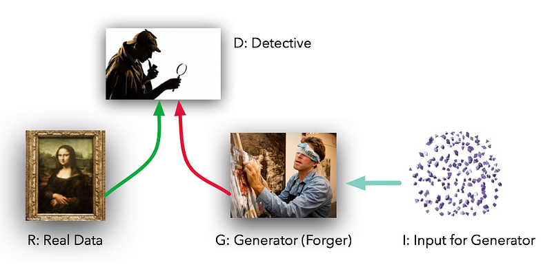
The models play two distinct (literally, adversarial) roles. Given some real data set R, G is the generator, trying to create fake data that looks just like the genuine data, while D is the discriminator, getting data from either the real set or G and labeling the difference. Goodfellow’s metaphor (and a fine one it is) was that G was like a team of forgers trying to match real paintings with their output, while D was the team of detectives trying to tell the difference. (Except that in this case, the forgers G never get to see the original data — only the judgments of D. They’re like blind forgers.)

In the ideal case, both D and G would get better over time until G had essentially become a “master forger” of the genuine article and D was at a loss, “unable to differentiate between the two distributions.”

In practice, what Goodfellow had shown was that G would be able to perform a form of unsupervised learning on the original dataset, finding some way of representing that data in a (possibly) much lower-dimensional manner. And as Yann LeCun famously stated, unsupervised learning is the “cake” of true AI.

---

This powerful technique seems like it must require a metric ton of code just to get started, right? Nope. Using PyTorch, we can actually create a very simple GAN in under 50 lines of code. There are really only 5 components to think about:

• R: The original, genuine data set
• I: The random noise that goes into the generator as a source of entropy
• G: The generator which tries to copy/mimic the original data set
• D: The discriminator which tries to tell apart G’s output from R
• The actual ‘training’ loop where we teach G to trick D and D to beware G.

1.) R: In our case, we’ll start with the simplest possible R — a bell curve. This function takes a mean and a standard deviation and returns a function which provides the right shape of sample data from a Gaussian with those parameters. In our sample code, we’ll use a mean of 4.0 and a standard deviation of 1.25.

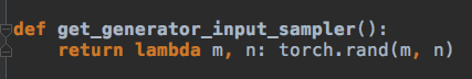
2.) I: The input into the generator is also random, but to make our job a little bit harder, let’s use a uniform distribution rather than a normal one. This means that our model G can’t simply shift/scale the input to copy R, but has to reshape the data in a non-linear way.

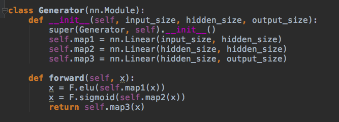
3.) G: The generator is a standard feedforward graph — two hidden layers, three linear maps. We’re using an ELU (exponential linear unit) because they’re the new black, yo. G is going to get the uniformly distributed data samples from I and somehow mimic the normally distributed samples from R.

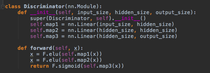
4.) D: The discriminator code is very similar to G’s generator code; a feedforward graph with two hidden layers and three linear maps. It’s going to get samples from either R or G and will output a single scalar between 0 and 1, interpreted as ‘fake’ vs. ‘real’. This is about as milquetoast as a neural net can get.

5.) Finally, the training loop alternates between two modes: first training D on real data vs. fake data, with accurate labels (think of this as Police Academy); and then training G to fool D, with inaccurate labels (this is more like those preparation montages from Ocean’s Eleven). It’s a fight between good and evil, people.

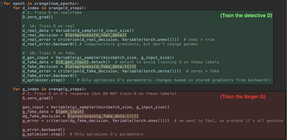
Even if you haven’t seen PyTorch before, you can probably tell what’s going on. In the first (green) section, we push both types of data through D and apply a differentiable criterion to D’s guesses vs. the actual labels. That pushing is the ‘forward’ step; we then call ‘backward()’ explicitly in order to calculate gradients, which are then used to update D’s parameters in the d_optimizer step() call. G is used but isn’t trained here.

Then in the last (red) section, we do the same thing for G — note that we also run G’s output through D (we’re essentially giving the forger a detective to practice on) but we do not optimize or change D at this step. We don’t want the detective D to learn the wrong labels. Hence, we only call g_optimizer.step().

And…that’s all. There’s some other boilerplate code but the GAN-specific stuff is just those 5 components, nothing else.

---

After a few thousand rounds of this forbidden dance between D and G, what do we get? The discriminator D gets good very quickly (while G slowly moves up), but once it gets to a certain level of power, G has a worthy adversary and begins to improve. Really improve.

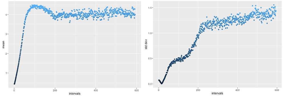
Over 20,000 training rounds, the mean of G’s output overshoots 4.0 but then comes back in a fairly stable, correct range (left). Likewise, the standard deviation initially drops in the wrong direction but then rises up to the desired 1.25 range (right), matching R.

Ok, so the basic stats match R, eventually. How about the higher moments? Does the shape of the distribution look right? After all, you could certainly have a uniform distribution with a mean of 4.0 and a standard deviation of 1.25, but that wouldn’t really match R. Let’s show the final distribution emitted by G.

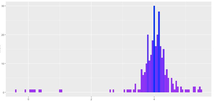
Not bad. The left tail is a bit longer than the right, but the skew and kurtosis are, shall we say, evocative of the original Gaussian.

G recovers the original distribution R nearly perfectly — and D is left cowering in the corner, mumbling to itself, unable to tell fact from fiction. This is precisely the behavior we want (see Figure 1 in Goodfellow). From fewer than 50 lines of code.

Goodfellow would go on to publish many other papers on GANs, including a 2016 gem describing some practical improvements, including the minibatch discrimination method adapted here. And here’s a 2-hour tutorial he presented at NIPS 2016. For TensorFlow users, here’s a parallel post from Aylien on GANs.

Ok. Enough talk. Go look at the code.