


由于不断变化的需求和现代化基础设施的动态性质,为大型应用程序规划容量可能会非常困难。例如,传统的反应式方法依赖于某些 DevOps 指标(如 CPU 和内存)的静态阈值,而这些指标在这样的环境中并不足以解决问题。在这篇文章中,我们展示了如何使用 Amazon SageMaker 内置算法,对存储在 Amazon Timestream 中的汇总 DevOps 数据(CPU、内存、每秒交易量)进行预测分析。这样可以实现主动式容量规划,防止潜在的业务中断。通过这种方法,您可以使用 Amazon SageMaker,对存储在 Amazon Timestream 中的任何时间序列数据运行机器学习。
Amazon Timestream 是一种快速、可扩展且无服务器的时间序列数据库服务,可轻松存储和分析每天数万亿个事件。Amazon Timestream 会自动纵向扩展或缩减以调整容量和性能,因此您无需管理底层基础设施。
Amazon SageMaker 是一项完全托管式机器学习(ML)服务。借助 Amazon SageMaker,数据科学家和开发人员可以轻松快速地构建和训练机器学习模型,然后直接将其部署到生产就绪型托管环境中。它提供了集成的 Jupyter 创作 Notebook 实例,可快速访问数据来源以进行探索和分析,因此您无需管理服务器。它还提供了常见的机器学习算法,这些算法经过优化,可高效地运行在分布式环境中的超大量数据上。
解决方案概览
DevOps 团队可以使用 Timestream 存储指标、日志和其它时间序列数据。然后,您可以查询这些数据,深入了解系统的行为。Timestream 能够以低延迟处理大量传入数据,这使团队能够执行实时分析。DevOps 团队可以实时分析性能指标和其它运营数据,以便快速制定决策。
以下参考架构展示了如何将 Timestream 用于 DevOps 应用场景。
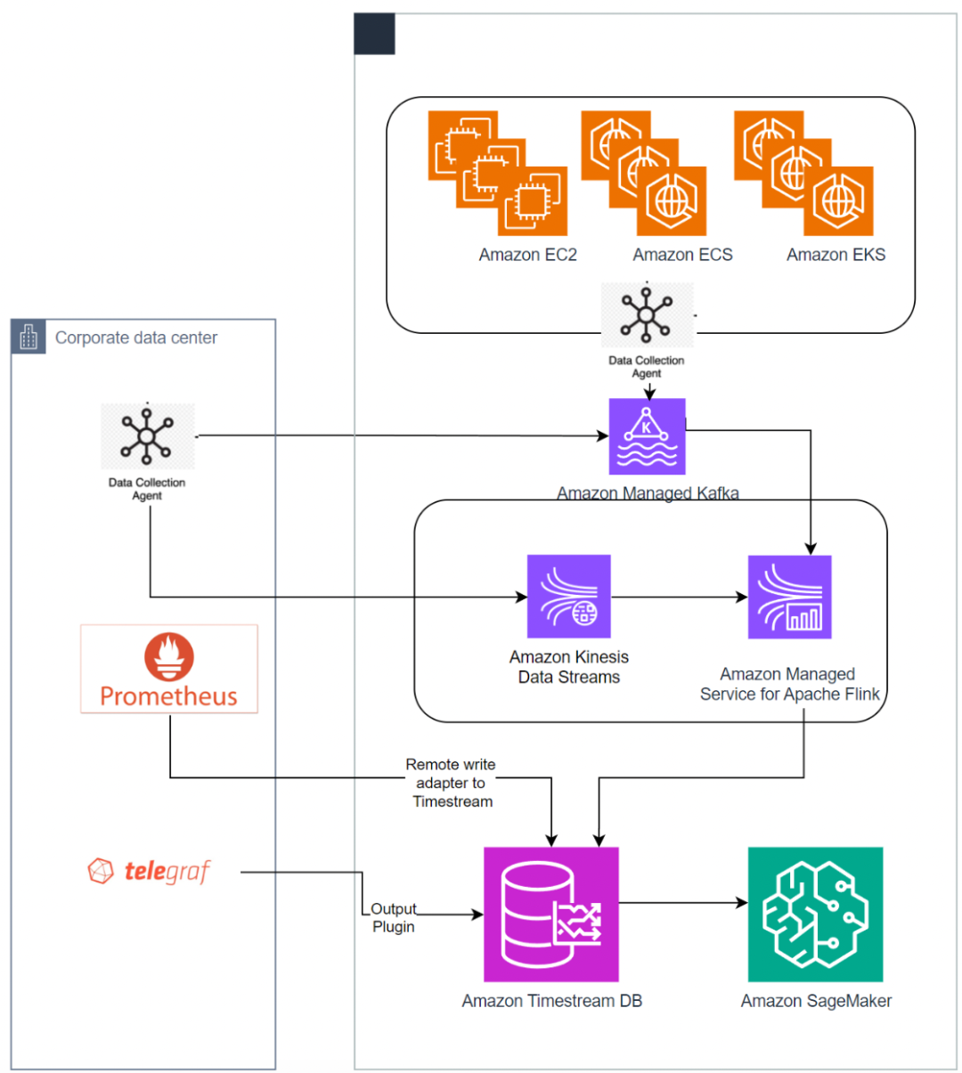
解决方案包含以下关键组件:
遥测数据,来自云端和本地运行的应用程序和服务器,使用开源收集代理(如 Prometheus 和 Telegraf)摄入。
数据也可以摄取自流式服务,例如 Amazon Managed Streaming for Apache Kafka (Amazon MSK) 和 Amazon Kinesis,使用适用于 Apache Flink 的亚马逊托管服务摄入。
摄取数据后,您可以使用可视化工具来分析数据和生成控制面板,这些工具包括 Grafana 和 Amazon QuickSight(有关详细信息,请参阅 Amazon QuickSight:
https://docs.aws.amazon.com/timestream/latest/developerguide/Quicksight.html),以及其它使用 JBDC 和 ODBC 驱动程序的工具。
Amazon SageMaker 用于运行预测分析。有关更多详细信息,请参阅 Amazon SageMaker:
https://docs.aws.amazon.com/timestream/latest/developerguide/Sagemaker.html
先决条件
要理解这篇文章,您应该熟悉 Timestream、Amazon SageMaker、Amazon Simple Storage Service (Amazon S3)、Amazon Identity and Access Management (IAM) 和 Python 的关键概念。这篇文章还包括一个动手试验室,使用 Amazon CloudFormation 模板和 Jupyter Notebook 预置,并与相关 Amazon 服务交互。这需要一个具有必要 IAM 权限的 Amazon 账户。
启动动手实验室
完成以下步骤以启动动手实验室:
1. 启动 CloudFormation 模板:
https://console.aws.amazon.com/cloudformation/home?#/stacks/create/review?templateURL=https://aws-blogs-artifacts-public.s3.amazonaws.com/artifacts/DBBLOG-3596/predictive_analytics.yaml
注意:此解决方案创建的亚马逊云科技资源会在账户中产生费用,请务必在完成后删除堆栈。
2. 提供堆栈名称,将所有其它选项保留为默认值。此堆栈创建 Timestream 数据库和表,并提取汇总 DevOps 数据示例。它还会创建一个 Amazon SageMaker Notebook 实例和 Amazon S3 存储桶。
3. 堆栈完成后,记下 Notebook 实例和 S3 存储桶的名称,这些信息在 Amazon CloudFormation 控制台上堆栈的输出选项卡中列出。
我们使用 Amazon SageMaker Notebook 实例来准备来自 Timestream 的数据、训练机器学习模型和运行预测。
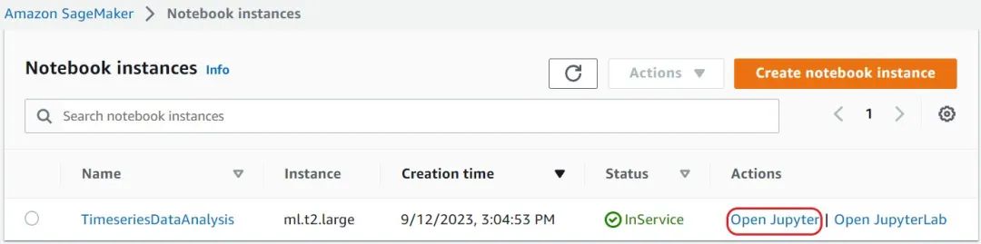
4. 要访问 Notebook 实例,请导航到 Amazon SageMaker 控制台,然后在导航窗格中选择 Notebook 实例。
5. 打开由 CloudFormation 堆栈创建的实例。
6. 当 Notebook 的状态为正在使用时,选择打开 Jupyter。
以下示例显示了一个名为 TimeseriesDataAnalysis 的 Notebook 实例。
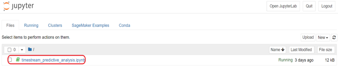
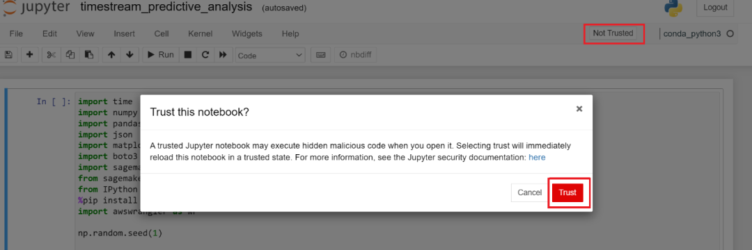
7. 选择
timestream_predictive_analysis.ipynb 并将其标记为可信。
准备数据用于分析
现在,您可以运行 Notebook 中的单元格,来开始分析数据并准备数据用于训练。请完成以下步骤:
1. 以下代码设置 Amazon SageMaker 会话并创建 Amazon S3 和 Timestream 客户端。它还安装 Amazon SageMaker Data Wrangler 库,该库将 Pandas 库的功能扩展到亚马逊云科技,连接 DataFrames 与亚马逊云科技数据和分析服务,从而为 Timestream 和许多其它亚马逊云科技服务提供快速集成。
import time
import numpy as np
import pandas as pd
import json
import matplotlib.pyplot as plt
import boto3
import sagemaker
from sagemaker import get_execution_role
from IPython import display
%pip install awswrangler
import awswrangler as wr


np.random.seed(1)


# 设置 Sagemaker 会话
prefix = "sagemaker/DEMO-deepar"
sagemaker_session = sagemaker.Session()
role = get_execution_role()
bucket = sagemaker_session.default_bucket()


# 设置 S3 存储桶路径来上传训练数据集
s3_data_path = f"{bucket}/{prefix}/data"
s3_output_path = f"{bucket}/{prefix}/output"
print(s3_data_path)
print(s3_output_path)


# 设置 S3 客户端
s3_client = boto3.client('s3')


# Timestream 配置。
DB_NAME = "Demo_Predictive_Analysis" # <--- 指定在 Amazon Timestream 中创建的数据库
TABLE_NAME = "Telemetry_Aggregated_Data" # <--- 指定在 Amazon Timestream 中创建的表


timestream_client = boto3.client('timestream-query')
2. 在此步骤结束时,记下 S3 存储桶路径的输出。
分析完成后,您可以删除这些存储桶
3. 从 Timestream 查询数据:
query = """
SELECT *
FROM "Demo_Predictive_Analysis"."Telemetry_Aggregated_Data"
"""


result = wr.timestream.query(sql=query,pagination_config={'PageSize': 1000})
display.display(result)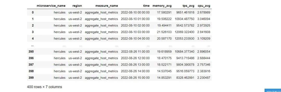
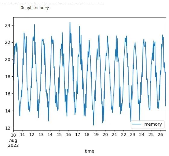
4. 可视化时间序列数据:
labels = ['cpu', 'memory', 'tps']
cpu_series = pd.Series(data = result['cpu_avg'].values, index = pd.to_datetime(result['time']))
memory_series = pd.Series(data = result['memory_avg'].values, index = pd.to_datetime(result['time']))
tps_series = pd.Series(data = result['tps_avg'].values, index = pd.to_datetime(result['time']))
## 收集列表中的所有序列
time_series = []
time_series.append(cpu_series)
time_series.append(memory_series)
time_series.append(tps_series)
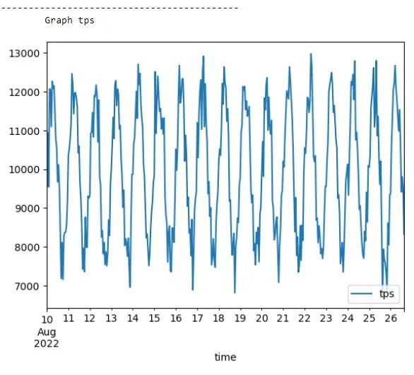
for k in range(len(time_series)):
print(f'-------------------------------------------\n\tGraph {labels[k]}')
time_series[k].plot(label = labels[k])
plt.legend(loc='lower right')
plt.show()以下是 CPU 使用率图。

以下是内存使用情况图。
以下是每秒事务数(TPS,Transactions Per Second)图。
解决方案使用 Amazon SageMaker DeepAR 预测算法,之所以选择该算法,是因为它使用循环神经网络(RNN,Recurrent Neural Network)来高效地预测一维时间序列数据。DeepAR 因其适应不同时间序列模式的能力而脱颖而出,这些特性使其成为一种多功能且强大的选择。它采用有监督学习方法,使用已标注的历史数据进行训练,并利用 RNN 架构的优势来捕获顺序数据中的时间依赖关系。
5. 使用以下 DeepAR 超参数来初始化机器学习实例:
freq = "H" ## 时间,以小时为单位
prediction_length = 48
context_length = 72
data_length = 400
num_ts = 2
period = 24


hyperparameters = {
    "time_freq": freq,
    "context_length": str(context_length),
    "prediction_length": str(prediction_length),
    "num_cells": "40",
    "num_layers": "3",
    "likelihood": "gaussian",
    "epochs": "20",
    "mini_batch_size": "32",
    "learning_rate": "0.001",
    "dropout_rate": "0.05",
    "early_stopping_patience": "10",
}
查看之前的图表,您会发现所有三个指标的模式看起来都相似。因此,我们只使用 CPU 指标进行训练。但是,我们可以使用训练后的模型来预测 CPU 之外的其它指标。如果数据模式不同,那么我们必须分别训练每个数据集并相应进行预测。
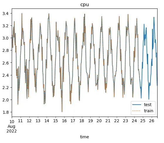
我们有大约 16 天的 24 小时周期内的数据。我们使用前 14 天的数据,在 3 天(72 小时)的上下文窗口中训练模型,并使用最后 2 天(48 小时)来测试我们的预测。
6. 训练数据是数据的前面部分,截止到最近 2 天(48 小时):
time_series_training = []
for ts in time_series:
    time_series_training.append(ts[:-prediction_length])
time_series[0].plot(label="test", title = "cpu")
time_series_training[0].plot(label="train", ls=":")
plt.legend()
plt.show()
下图显示了数据并将其与测试数据叠加显示。
7. 下一步根据 DeepAR 输入格式对数据进行格式化,以便将数据用于训练模型。然后,该步骤将数据集保存到 Amazon S3。
def series_to_obj(ts, cat=None):
    obj = {"start": str(ts.index[0]), "target": list(ts)}
    if cat is not None:
        obj["cat"] = cat
    return obj


def series_to_jsonline(ts, cat=None):
    return json.dumps(series_to_obj(ts, cat))


encoding = "utf-8"
FILE_TRAIN = "train.json"
FILE_TEST = "test.json"
with open(FILE_TRAIN, "wb") as f:
    for ts in time_series_training:
        f.write(series_to_jsonline(ts).encode(encoding))
        f.write("\n".encode(encoding))


with open(FILE_TEST, "wb") as f:
    for ts in time_series:
        f.write(series_to_jsonline(ts).encode(encoding))
        f.write("\n".encode(encoding))
s3 = boto3.client("s3")
s3.upload_file(FILE_TRAIN, bucket, prefix + "/data/train/" + FILE_TRAIN)
s3.upload_file(FILE_TEST, bucket, prefix + "/data/test/" + FILE_TRAIN)
您可以导航到 Amazon S3 控制台,然后查看先前创建的存储桶(例如 s3://sagemaker-<region>-<account_number>/sagemaker/DEMO-deepar/data)来验证文件 test.json 和 train.json。
使用 DeepAR 预测算法训练模型
此步骤使用通用估计器训练模型。它使用包含 DeepAR 算法的 SageMaker 镜像启动机器学习实例(实例类型为 ml.c4.xlarge):
image_uri = sagemaker.image_uris.retrieve("forecasting-deepar", boto3.Session().region_name)
estimator = sagemaker.estimator.Estimator(
sagemaker_session=sagemaker_session,
image_uri=image_uri,
role=role,
instance_count=1,
instance_type="ml.c4.xlarge",
base_job_name="DEMO-deepar",
output_path=f"s3://{s3_output_path}",
)
estimator.set_hyperparameters(**hyperparameters)
data_channels = {"train": f"s3://{s3_data_path}/train/", "test": f"s3://{s3_data_path}/test/"}
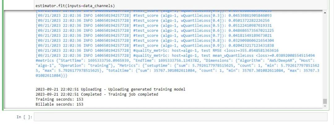
estimator.fit(inputs=data_channels)等待模型训练完成(大约 5 分钟),然后再运行预测。
当训练作业完成后,您将看到以下响应。
生成预测见解
当模型训练阶段成功完成后,下一步就是通过部署端点来启动预测实例。
1. 使用以下代码部署端点:
job_name = estimator.latest_training_job.name
endpoint_name = sagemaker_session.endpoint_from_job(
job_name=job_name,
initial_instance_count=1,
instance_type="ml.m4.xlarge",
image_uri=image_uri,
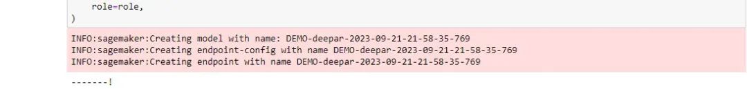
role=role,
)启动实例可能需要一段时间。最初,输出中只显示一个连字符(–)。等到状态行以感叹号(!)结尾。
2. 使用以下帮助程序类来运行预测:
class DeepARPredictor(sagemaker.predictor.RealTimePredictor):
def set_prediction_parameters(self, freq, prediction_length):
"""设置时间频率和预测长度参数。**必须** 调用此方法
然后才能使用“predict”。
Parameters:
freq -- 表示时间频率的字符串
prediction_length -- 整数,预测的时间点数量
返回值:无。
"""
self.freq = freq
self.prediction_length = prediction_length
def predict(
self,
ts,
cat=None,
encoding="utf-8",
num_samples=100,
quantiles=["0.1", "0.5", "0.9"],
content_type="application/json",
):
"""请求对“ts”中列出的时间序列进行预测,每个时间序列带有(可选)
对应的类别,在“cat”中列出。
Parameters:
ts -- “Pandas.Series”对象列表,要预测的时间序列
cat -- 整数列表(默认值:无)
encoding -- 字符串,用于请求的编码(默认值:“utf-8”)
num_samples -- 整数,预测时要计算的样本数(默认值:100)
quantiles -- 指定要计算的分位数的字符串列表(默认值:["0.1"、“0.5"、“0.9"])
返回值:“pandas.DataFrame”对象的列表,每个对象中包含预测
"""
prediction_times = [x.index[-1] + pd.Timedelta(1, unit=self.freq) for x in ts]
req = self.__encode_request(ts, cat, encoding, num_samples, quantiles)
res = super(DeepARPredictor, self).predict(req, initial_args={"ContentType": content_type})
return self.__decode_response(res, prediction_times, encoding)
def __encode_request(self, ts, cat, encoding, num_samples, quantiles):
instances = [series_to_obj(ts[k], cat[k] if cat else None) for k in range(len(ts))]
configuration = {
"num_samples": num_samples,
"output_types": ["quantiles"],
"quantiles": quantiles,
}
http_request_data = {"instances": instances, "configuration": configuration}
return json.dumps(http_request_data).encode(encoding)
def __decode_response(self, response, prediction_times, encoding):
response_data = json.loads(response.decode(encoding))
list_of_df = []
for k in range(len(prediction_times)):
prediction_index = pd.date_range(
start=prediction_times[k], freq=self.freq, periods=self.prediction_length
)
list_of_df.append(
pd.DataFrame(
data=response_data["predictions"][k]["quantiles"], index=prediction_index
)
)
return list_of_df
predictor = DeepARPredictor(endpoint_name=endpoint_name, sagemaker_session=sagemaker_session)
predictor.set_prediction_parameters(freq, prediction_length)
list_of_df = predictor.predict(time_series_training[:3], content_type="application/json")
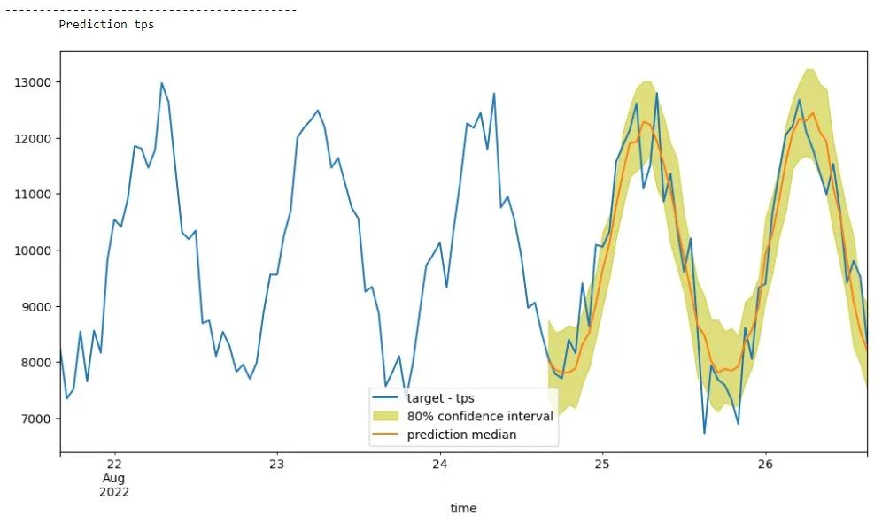
actual_data = time_series[:3]3. 最后,您可以将结果可视化:
for k in range(len(list_of_df)):
print(f'-------------------------------------------\n\tPrediction {labels[k]}')
plt.figure(figsize=(12, 6))
actual_data[k][-prediction_length - context_length :].plot(label=f'target - {labels[k]}')
p10 = list_of_df[k]["0.1"]
p90 = list_of_df[k]["0.9"]
plt.fill_between(p10.index, p10, p90, color="y", alpha=0.5, label="80% confidence interval")
list_of_df[k]["0.5"].plot(label="prediction median")
plt.legend()
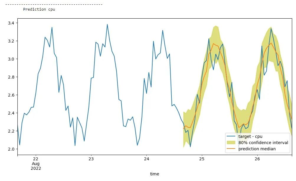
plt.show()下图显示了我们的 CPU 预测。
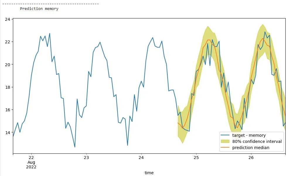
下图显示了我们的内存预测。
下图显示了我们的 TPS 预测。
4. 删除端点
sagemaker_session.delete_endpoint(endpoint_name)我们的预测结果与测试数据非常吻合,可以使用这些预测数据来规划容量。您可以按照本文中的步骤,无缝地扩展此解决方案,用于预测存储在 Timestream 中的其它时间序列数据。如果用户希望在现实场景中对一系列时间序列数据集进行准确预测,可以使用这种灵活且适用的解决方案。
Timestream 中的汇总
通常,最佳做法是在训练模型之前,以较低的频率汇总时间序列数据。使用原始数据会使模型运行缓慢且导致准确性降低。
使用 Timestream 计划查询功能,您可以汇总数据并将数据存储在不同的 Timestream 表中。您可以为业务报告使用计划查询,汇总应用程序中的最终用户活动,因此您可以训练机器学习模型来提供个性化的数据。您还可以使用计划查询提供警报,检测异常、网络入侵或欺诈活动,这样就可以立即采取补救措施。以下是 SQL 查询示例,该查询可以作为计划查询运行,以在 1 小时的时间间隔内汇总/向上采样数据:
select
microservice_name,
region,
'aggregate_host_metric' as measure_name,
bin(time, 1h) as time,
round(avg(memory),2) as memory_avg,
round(avg(tps),2) as tps_avg,
round(avg(cpu),2) as cpu_avg
from “Demo”.”source_metrics”
group by microservice_name, region, bin(time, 1h)
清理
为避免产生费用,请使用亚马逊云科技管理控制台删除您在运行本练习时创建的资源:http://aws.amazon.com/console
删除在 CloudFormation 堆栈之外创建的 Amazon SageMaker 资源和 Amazon S3 存储桶。
清空创建的 Amazon S3 存储桶,这样在删除堆栈时就不会遇到问题。
删除为此解决方案创建的 CloudFormation 堆栈。
结论
在这篇文章中,我们向您演示了如何使用 Amazon SageMaker DeepAR 算法,对存储在 Timestream 中的 DevOps 时间序列数据运行预测分析,用于改善容量规划。通过结合 Amazon SageMaker 和 Timestream 的功能,您可以对时间序列数据集进行预测并获得宝贵的见解。
有关时间流聚合的更多信息,请参阅 Queries with aggregate functions(使用聚合函数进行查询):
https://docs.aws.amazon.com/timestream/latest/developerguide/sample-queries.iot-scenarios.html
有关高级时间序列分析函数,请参阅 Time-series functions(时间序列函数):
https://docs.aws.amazon.com/timestream/latest/developerguide/timeseries-specific-constructs.functions.html
要了解有关使用 DeepAR 算法的更多信息,请参阅使用 DeepAR 算法的最佳实践:
https://docs.aws.amazon.com/sagemaker/latest/dg/deepar.html#deepar_best_practices
本篇作者

Bobilli Balwanth
亚马逊云科技 Timestream SA,常驻犹他州。在加入亚马逊云科技之前,他曾在 Goldman Sachs 担任 Cloud Database Architect。他对数据库和云计算充满热情。对于在云端构建安全、可扩展和弹性的解决方案(尤其是云数据库)这个领域,他拥有丰富的经验。

Norbert Funke
亚马逊云科技 Timestream SA,常驻纽约。在加入亚马逊云科技之前,他曾在 PwC 旗下的一家数据咨询公司,从事有关数据架构和数据分析方面的工作。

Renuka Uttarala
亚马逊云科技资深 Neptune/Timestream SA,领导专门研究数据服务架构解决方案的全球团队。她拥有 20 多年的 IT 行业经验,专门从事高级分析和数据科学领域。在加入亚马逊云科技之前,她曾在多家公司担任产品开发、企业架构和解决方案工程领导职务,包括 HCL Technologies、Amdocs Openet、Warner Bros、Discovery 和 Oracle Corporation。

星标不迷路,开发更极速!
关注后记得星标「亚马逊云开发者」

听说,点完下面4个按钮
就不会碰到bug了!


 8474
8474


 被折叠的 条评论
为什么被折叠?
被折叠的 条评论
为什么被折叠?
 到【灌水乐园】发言


