数据埋点系列 17｜ 预测分析和预测模型：用数据洞察未来

在数据驱动的决策时代，预测分析和预测模型已成为组织的重要战略工具。通过分析历史数据，我们可以预测未来趋势，做出更明智的决策。本文将深入探讨预测分析的核心概念、常用技术和实际应用。

1. 预测分析的基础

预测分析是使用历史数据、统计算法和机器学习技术来识别未来结果的可能性的过程。

1.1 预测分析的类型

1. 分类预测：预测离散的类别
2. 回归预测：预测连续的数值
3. 时间序列预测：基于时间序列数据进行预测

import pandas as pd
import numpy as np
from sklearn.model_selection import train_test_split
from sklearn.metrics import classification_report, mean_squared_error
from sklearn.linear_model import LogisticRegression, LinearRegression
from statsmodels.tsa.arima.model import ARIMA

class PredictiveAnalytics:
    def __init__(self):
        pass
    
    def classification_prediction(self, X, y):
        X_train, X_test, y_train, y_test = train_test_split(X, y, test_size=0.2, random_state=42)
        model = LogisticRegression()
        model.fit(X_train, y_train)
        y_pred = model.predict(X_test)
        print(classification_report(y_test, y_pred))
    
    def regression_prediction(self, X, y):
        X_train, X_test, y_train, y_test = train_test_split(X, y, test_size=0.2, random_state=42)
        model = LinearRegression()
        model.fit(X_train, y_train)
        y_pred = model.predict(X_test)
        mse = mean_squared_error(y_test, y_pred)
        print(f"Mean Squared Error: {mse}")
    
    def time_series_prediction(self, data, order=(1,1,1)):
        model = ARIMA(data, order=order)
        results = model.fit()
        forecast = results.forecast(steps=5)
        print("Forecasted values:")
        print(forecast)

# 使用示例
analytics = PredictiveAnalytics()

# 分类预测
X_class = np.random.rand(100, 2)
y_class = np.random.choice([0, 1], 100)
analytics.classification_prediction(X_class, y_class)

# 回归预测
X_reg = np.random.rand(100, 1)
y_reg = 2 * X_reg + 1 + np.random.randn(100, 1) * 0.1
analytics.regression_prediction(X_reg, y_reg)

# 时间序列预测
time_series_data = pd.Series(np.random.randn(100))
analytics.time_series_prediction(time_series_data)

2. 高级预测模型

除了基本的预测模型，还有许多高级模型可以处理更复杂的预测任务。

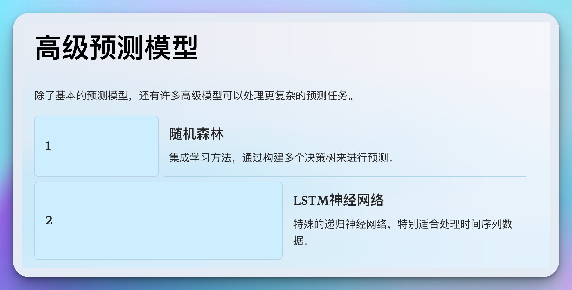
2.1 随机森林

随机森林是一种集成学习方法，通过构建多个决策树来进行预测。

from sklearn.ensemble import RandomForestRegressor
from sklearn.datasets import make_regression

def random_forest_prediction():
    X, y = make_regression(n_samples=100, n_features=4, noise=0.1)
    X_train, X_test, y_train, y_test = train_test_split(X, y, test_size=0.2, random_state=42)
    
    model = RandomForestRegressor(n_estimators=100, random_state=42)
    model.fit(X_train, y_train)
    
    y_pred = model.predict(X_test)
    mse = mean_squared_error(y_test, y_pred)
    print(f"Random Forest Mean Squared Error: {mse}")
    
    feature_importance = model.feature_importances_
    for i, importance in enumerate(feature_importance):
        print(f"Feature {i+1} importance: {importance}")

random_forest_prediction()

2.2 LSTM神经网络

长短期记忆（LSTM）网络是一种特殊的递归神经网络，特别适合处理时间序列数据。

from tensorflow.keras.models import Sequential
from tensorflow.keras.layers import LSTM, Dense
from sklearn.preprocessing import MinMaxScaler

def lstm_prediction():
    # 生成示例时间序列数据
    time_steps = np.linspace(0, 100, 1000)
    data = np.sin(time_steps) + np.random.normal(0, 0.1, 1000)
    
    # 数据预处理
    scaler = MinMaxScaler()
    data_scaled = scaler.fit_transform(data.reshape(-1, 1))
    
    # 准备训练数据
    def create_sequences(data, seq_length):
        sequences = []
        targets = []
        for i in range(len(data) - seq_length):
            seq = data[i:i+seq_length]
            target = data[i+seq_length]
            sequences.append(seq)
            targets.append(target)
        return np.array(sequences), np.array(targets)
    
    seq_length = 50
    X, y = create_sequences(data_scaled, seq_length)
    X = X.reshape((X.shape[0], X.shape[1], 1))
    
    # 构建LSTM模型
    model = Sequential([
        LSTM(50, activation='relu', input_shape=(seq_length, 1)),
        Dense(1)
    ])
    model.compile(optimizer='adam', loss='mse')
    
    # 训练模型
    model.fit(X, y, epochs=50, batch_size=32, verbose=0)
    
    # 预测
    last_sequence = data_scaled[-seq_length:]
    next_prediction = model.predict(last_sequence.reshape(1, seq_length, 1))
    next_prediction = scaler.inverse_transform(next_prediction)
    
    print(f"Next predicted value: {next_prediction[0][0]}")

lstm_prediction()

3. 特征工程

特征工程是预测建模中最重要的步骤之一，它可以显著提高模型的性能。

import pandas as pd
import numpy as np
from sklearn.preprocessing import StandardScaler, OneHotEncoder
from sklearn.impute import SimpleImputer
from sklearn.compose import ColumnTransformer
from sklearn.pipeline import Pipeline

def feature_engineering(data):
    # 假设我们有一个包含数值和分类特征的数据集
    numeric_features = ['age', 'income']
    categorical_features = ['gender', 'occupation']
    
    # 创建预处理管道
    numeric_transformer = Pipeline(steps=[
        ('imputer', SimpleImputer(strategy='median')),
        ('scaler', StandardScaler())
    ])
    
    categorical_transformer = Pipeline(steps=[
        ('imputer', SimpleImputer(strategy='constant', fill_value='missing')),
        ('onehot', OneHotEncoder(handle_unknown='ignore'))
    ])
    
    preprocessor = ColumnTransformer(
        transformers=[
            ('num', numeric_transformer, numeric_features),
            ('cat', categorical_transformer, categorical_features)
        ])
    
    # 拟合和转换数据
    X_processed = preprocessor.fit_transform(data)
    
    # 获取特征名称
    feature_names = (numeric_features +
                     preprocessor.named_transformers_['cat']
                     .named_steps['onehot']
                     .get_feature_names(categorical_features).tolist())
    
    return pd.DataFrame(X_processed, columns=feature_names)

# 使用示例
data = pd.DataFrame({
    'age': [25, 30, np.nan, 40],
    'income': [50000, 60000, 75000, np.nan],
    'gender': ['M', 'F', 'M', 'F'],
    'occupation': ['engineer', 'teacher', np.nan, 'doctor']
})

processed_data = feature_engineering(data)
print(processed_data)

4. 模型评估和选择

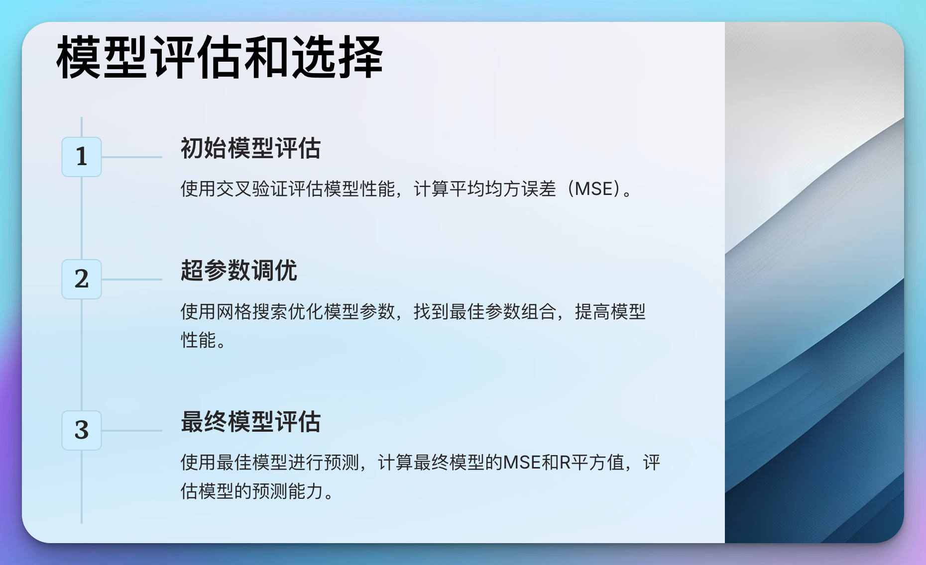
选择合适的模型并正确评估其性能是预测分析中的关键步骤。

from sklearn.model_selection import cross_val_score, GridSearchCV
from sklearn.ensemble import RandomForestRegressor
from sklearn.metrics import mean_squared_error, r2_score

def model_evaluation_and_selection(X, y):
    # 初始模型评估
    model = RandomForestRegressor(random_state=42)
    scores = cross_val_score(model, X, y, cv=5, scoring='neg_mean_squared_error')
    mse_scores = -scores
    print(f"Cross-validation MSE scores: {mse_scores}")
    print(f"Average MSE: {np.mean(mse_scores)}")
    
    # 超参数调优
    param_grid = {
        'n_estimators': [100, 200, 300],
        'max_depth': [None, 10, 20, 30],
        'min_samples_split': [2, 5, 10]
    }
    
    grid_search = GridSearchCV(model, param_grid, cv=5, scoring='neg_mean_squared_error')
    grid_search.fit(X, y)
    
    print(f"Best parameters: {grid_search.best_params_}")
    print(f"Best cross-validation score: {-grid_search.best_score_}")
    
    # 最终模型评估
    best_model = grid_search.best_estimator_
    y_pred = best_model.predict(X)
    mse = mean_squared_error(y, y_pred)
    r2 = r2_score(y, y_pred)
    
    print(f"Final model MSE: {mse}")
    print(f"Final model R-squared: {r2}")

# 使用示例
X, y = make_regression(n_samples=100, n_features=4, noise=0.1)
model_evaluation_and_selection(X, y)

5. 预测结果的应用

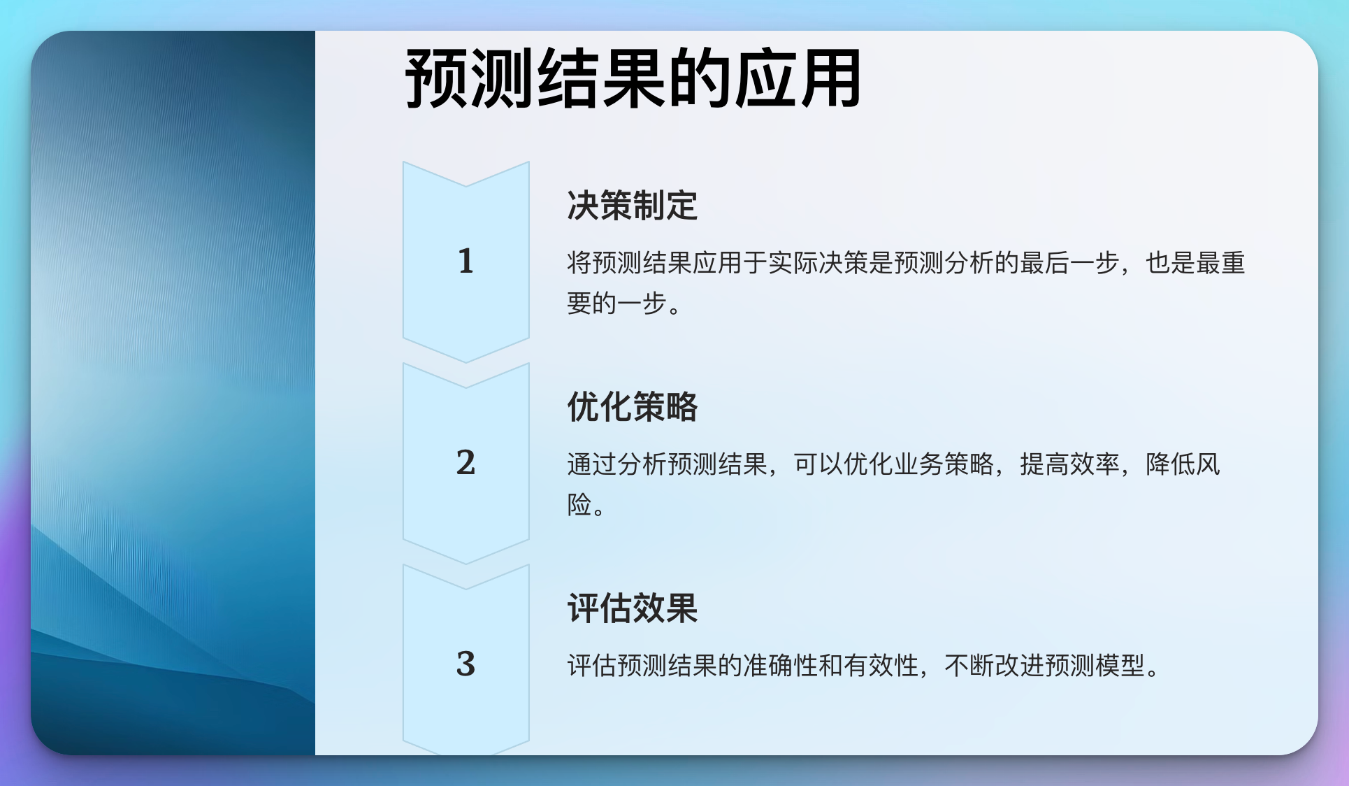
将预测结果应用于实际决策是预测分析的最后一步，也是最重要的一步。

import numpy as np
import matplotlib.pyplot as plt

class BusinessDecisionMaker:
    def __init__(self, predictions, actual_values, costs, revenues):
        self.predictions = predictions
        self.actual_values = actual_values
        self.costs = costs
        self.revenues = revenues
    
    def calculate_profit(self, threshold):
        decisions = (self.predictions >= threshold).astype(int)
        true_positives = np.sum((decisions == 1) & (self.actual_values == 1))
        false_positives = np.sum((decisions == 1) & (self.actual_values == 0))
        
        profit = true_positives * self.revenues - false_positives * self.costs
        return profit
    
    def find_optimal_threshold(self):
        thresholds = np.linspace(0, 1, 100)
        profits = [self.calculate_profit(t) for t in thresholds]
        optimal_threshold = thresholds[np.argmax(profits)]
        max_profit = np.max(profits)
        
        return optimal_threshold, max_profit
    
    def plot_profit_curve(self):
        thresholds = np.linspace(0, 1, 100)
        profits = [self.calculate_profit(t) for t in thresholds]
        
        plt.figure(figsize=(10, 6))
        plt.plot(thresholds, profits)
        plt.title('Profit vs Decision Threshold')
        plt.xlabel('Threshold')
        plt.ylabel('Profit')
        plt.grid(True)
        plt.show()

# 使用示例
predictions = np.random.rand(1000)
actual_values = np.random.randint(0, 2, 1000)
costs = 100
revenues = 500

decision_maker = BusinessDecisionMaker(predictions, actual_values, costs, revenues)
optimal_threshold, max_profit = decision_maker.find_optimal_threshold()

print(f"Optimal decision threshold: {optimal_threshold:.2f}")
print(f"Maximum profit: ${max_profit:.2f}")

decision_maker.plot_profit_curve()

6. 预测分析的挑战和局限性

尽管预测分析强大，但我们也需要认识到它的一些挑战和局限性：

1. 数据质量问题
2. 过拟合风险
3. 模型解释性
4. 预测偏差
5. 处理不确定性

class PredictiveAnalyticsChallenges:
    def __init__(self):
        self.challenges = [
            "数据质量问题",
            "过拟合风险",
            "模型解释性",
            "预测偏差",
            "处理不确定性"
        ]
    
    def discuss_challenge(self, challenge):
        if challenge in self.challenges:
            print(f"讨论预测分析的挑战: {challenge}")
            # 这里可以添加具体的讨论内容
        else:
            print(f"未知的挑战: {challenge}")
    
    def propose_solution(self, challenge):
        solutions = {
            "数据质量问题": "实施严格的数据清洗和验证流程",
            "过拟合风险": "使用交叉验证和正则化技术",
            "模型解释性": "采用可解释的AI技术，如SHAP值",
            "预测偏差": "定期监控和校准模型",
            "处理不确定性": "使用概率预测和置信区间"
        }
        if challenge in solutions:
            print(f"针对'{challenge}'的解决方案: {solutions[challenge]}")
        else:
            print(f"未找到针对'{challenge}'的解决方案")

# 使用示例
challenges = PredictiveAnalyticsChallenges()
challenges.discuss_challenge("模型解释性")
challenges.propose_solution("模型解释性")

7. 预测分析的未来趋势

预测分析领域正在快速发展，以下是一些值得关注的未来趋势：

1. 自动机器学习（AutoML）
2. 深度学习在预测分析中的应用
3. 边缘计算和实时预测
4. 可解释人工智能（XAI）
5. 联邦学习

class PredictiveAnalyticsTrends:
    def __init__(self):
        self.trends = [
            "自动机器学习（AutoML）",
            "深度学习在预测分析中的应用",
            "边缘计算和实时预测",
            "可解释人工智能（XAI）",
            "联邦学习"
        ]
    
    def explore_trend(self, trend):
        if trend in self.trends:
            print(f"\n探索预测分析的未来趋势: {trend}")
            impact = input("预期影响 (低/中/高): ")
            readiness = input("行业准备程度 (低/中/高): ")
            
            print(f"趋势分析结果:")
            print(f"  预期影响: {impact}")
            print(f"  行业准备程度: {readiness}")
            
            if impact.lower() == "高" and readiness.lower() != "高":
                print("  建议: 需要加大投资和关注以提高准备程度")
            elif impact.lower() == "中" and readiness.lower() == "低":
                print("  建议: 需要开始规划和准备")
            else:
                print("  建议: 持续关注发展动态")
        else:
            print(f"未知的预测分析趋势: {trend}")

# 使用示例
trends = PredictiveAnalyticsTrends()
trends.explore_trend("自动机器学习（AutoML）")

8. 案例研究：零售业的需求预测

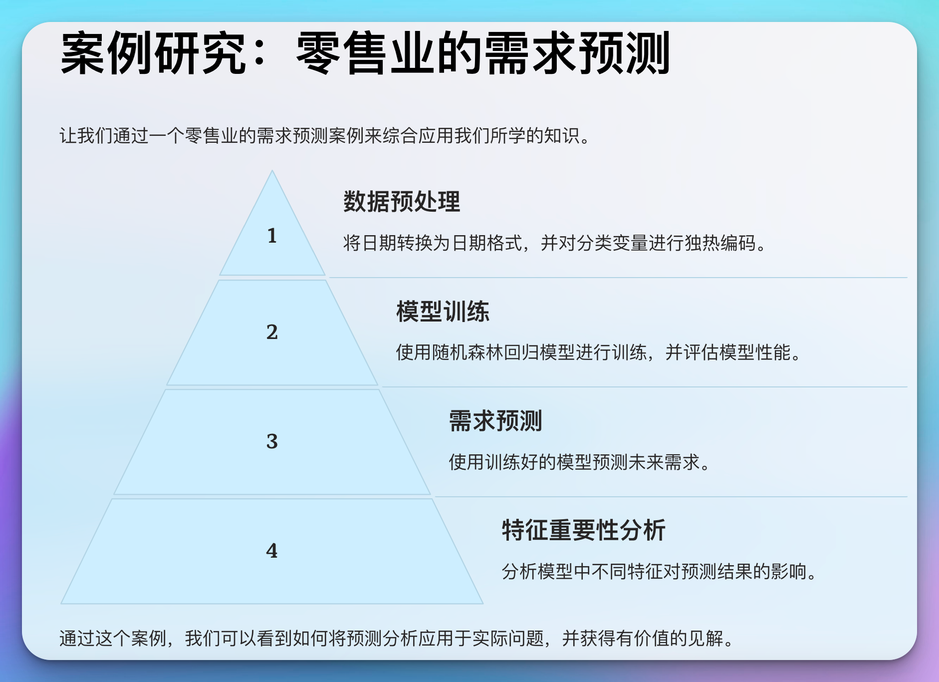
让我们通过一个零售业的需求预测案例来综合应用我们所学的知识。

import pandas as pd
import numpy as np
from sklearn.model_selection import train_test_split
from sklearn.ensemble import RandomForestRegressor
from sklearn.metrics import mean_squared_error, r2_score
import matplotlib.pyplot as plt

class RetailDemandForecasting:
    def __init__(self, data):
        self.data = data
        self.model = None
    
    def preprocess_data(self):
        # 假设数据包含 'date', 'product_id', 'store_id', 'sales', 'price', 'promotion'
        self.data['date'] = pd.to_datetime(self.data['date'])
        self.data['day_of_week'] = self.data['date'].dt.dayofweek
        self.data['month'] = self.data['date'].dt.month
        self.data['year'] = self.data['date'].dt.year
        
        # 对分类变量进行独热编码
        self.data = pd.get_dummies(self.data, columns=['product_id', 'store_id'])
        
        self.X = self.data.drop(['date', 'sales'], axis=1)
        self.y = self.data['sales']
    
    def train_model(self):
        X_train, X_test, y_train, y_test = train_test_split(self.X, self.y, test_size=0.2, random_state=42)
        
        self.model = RandomForestRegressor(n_estimators=100, random_state=42)
        self.model.fit(X_train, y_train)
        
        y_pred = self.model.predict(X_test)
        mse = mean_squared_error(y_test, y_pred)
        r2 = r2_score(y_test, y_pred)
        
        print(f"Mean Squared Error: {mse}")
        print(f"R-squared Score: {r2}")
    
    def forecast_demand(self, future_data):
        return self.model.predict(future_data)
    
    def plot_feature_importance(self):
        feature_importance = self.model.feature_importances_
        features = self.X.columns
        importance_df = pd.DataFrame({'feature': features, 'importance': feature_importance})
        importance_df = importance_df.sort_values('importance', ascending=False).head(10)
        
        plt.figure(figsize=(10, 6))
        plt.bar(importance_df['feature'], importance_df['importance'])
        plt.title('Top 10 Feature Importance')
        plt.xlabel('Features')
        plt.ylabel('Importance')
        plt.xticks(rotation=45, ha='right')
        plt.tight_layout()
        plt.show()

# 使用示例
# 生成模拟数据
np.random.seed(42)
dates = pd.date_range(start='2022-01-01', end='2022-12-31')
products = ['A', 'B', 'C']
stores = ['S1', 'S2']

data = []
for date in dates:
    for product in products:
        for store in stores:
            sales = np.random.randint(50, 200)
            price = np.random.uniform(10, 50)
            promotion = np.random.choice([0, 1], p=[0.7, 0.3])
            data.append([date, product, store, sales, price, promotion])

df = pd.DataFrame(data, columns=['date', 'product_id', 'store_id', 'sales', 'price', 'promotion'])

# 创建和使用需求预测模型
forecasting = RetailDemandForecasting(df)
forecasting.preprocess_data()
forecasting.train_model()
forecasting.plot_feature_importance()

# 预测未来需求
future_data = forecasting.X.iloc[-1:].copy()
future_data['day_of_week'] = (future_data['day_of_week'] + 1) % 7
future_data['price'] = 45  # 假设价格变化
future_demand = forecasting.forecast_demand(future_data)
print(f"预测的未来需求: {future_demand[0]:.2f}")

结语

预测分析和预测模型是数据驱动决策的核心工具，它们能够帮助组织洞察未来趋势，做出更明智的决策。本文探讨了预测分析的基础知识、高级模型、特征工程技巧、模型评估方法，以及如何将预测结果应用于实际决策。我们还讨论了预测分析面临的挑战和未来趋势。

关键要点包括：

1. 选择合适的预测模型对于特定问题至关重要
2. 特征工程可以显著提高模型性能
3. 正确的模型评估和选择是确保预测准确性的关键
4. 将预测结果转化为可操作的业务决策是预测分析的最终目标
5. 认识到预测分析的局限性，并采取措施应对相关挑战
6. 持续关注和适应预测分析领域的新趋势和技术进步

通过掌握这些预测分析和预测模型的知识和技能，数据科学家和分析师可以为组织创造巨大的价值，帮助组织在不确定的未来中做出更好的决策。记住，预测分析不仅仅是技术，更是将数据洞察转化为业务价值的艺术。通过不断学习和实践，你可以成为这个快速发展领域的专家，为组织的成功做出重要贡献。