负数与复数 | 不同时期的诠释与数理应用

注：机翻，未校。

---

On the history of negative and complex numbers’ interpretation

论负数和复数解释的历史

Galina I. Sinkevich

https://orcid.org/0000-0002-8595-1686

Saint Petersburg State University of Architecture and Civil Engineering, (Saint-Petersburg, Russia)

Abstract

摘要

The development of the concept of complex numbers from the $16^{th}$ to $19^{th}$ centuries. The origin and refinement of the geometric and physical meaning of complex numbers, the emergence of vectoral analysis.
复数概念从 16 世纪到 19 世纪的发展历程。复数的几何和物理意义的起源与完善，向量分析的出现。

Keywords

关键词

Complex number; quaternion; vector; Cardano; Bombelli; Wallis; Moivre; Euler; d’Alembert; Wessel; Argand; Gauss; Grassmann; Hamilton; Hankel
复数；四元数；向量；卡尔达诺；邦贝利；沃利斯；棣莫弗；欧拉；达朗贝尔；韦塞尔；阿尔冈；高斯；格拉斯曼；哈密顿；汉克尔

The development of the concept of numbers has a long history.

数的概念的发展有着悠久的历史。

In antiquity, only natural numbers were called numbers: 1, 2, 3, …, and aliquot fractions and proportions (ratios of natural numbers) were known.
在古代，只有自然数被称为数 ：1 、2 、3 ，…… ，并且已知整数的分数和比例（自然数的比）。

In Ancient Greece, it was discovered that values existed which could not be expressed in any ratio, for example the diagonal of the square of one.
在古希腊，人们发现存在一些量，无法用任何比例来表示，例如边长为 1 的正方形的对角线。

They were calculated approximately, using the method of exhaustion.
人们用穷竭法对它们进行近似计算。

The coefficients of equations, the roots of the equations could only be positive.
方程的系数、方程的根只能是正数。

If in solving tasks, a negative value arose, it was considered to be meaningless, as this quantity could not be less than nothing.
如果在解决问题时出现了负值，就会被认为是没有意义的，因为这个量不可能小于零。

Sometimes people said that in the commercial sense it could mean a debt.
有时人们说，从商业意义上讲，它可能意味着债务。

In Russian in the $18^{th}$ century negative numbers were called losses.
在 18 世纪的俄罗斯，负数被称为损失 。

So in solving equations, only positive roots were looked for.
所以在解方程时，人们只寻找正根。

This was how things were until the Renaissance.
这在文艺复兴之前一直是这样。

A negative number was also not recognized as a proper mathematical entity

负数也不被认为是一种恰当的数学实体

because for values, the rule of ratio had to be carried out: if the left part is a ratio that is less than the greater one, then the right part of the ratio should also be a ratio of the lesser to the greater.
因为对于数值来说，必须遵循比例规则 ：如果左边部分的比例小于较大的比例，那么右边部分的比例也应该是较小与较大的比例。

But for ratios of the kind $1:\frac{-1}{1}=\frac{1}{-1}$, there is no meaning, whether this related to natural or rational numbers.
但是对于像 $1:\frac{-1}{1}=\frac{1}{-1}$ 这样的比例，无论与自然数还是有理数相关，都毫无意义。

In 1494, Luca Pacioli (1445–1517) wrote the treatise Summa de arithmetica, geometria, proportioni et proportionalità (The sum of arithmetic, geometry, proportions and proportionality)

1494 年，卢卡・帕乔利（1445 - 1517）撰写了论文《算术、几何、比例和比例性大全》

in which he collected the knowledge of arithmetic held by Europeans and Indians.
在其中，他收集了欧洲人和印度人所掌握的算术知识。

In 1544, Michael Stifel was the first to state that negative numbers were numbers less than zero (below zero).

1544 年，迈克尔・施蒂费尔首次指出负数是小于零（零点以下）的数

Since this time, the concept of the numerical scale gradually began to form, in which positive numbers are located to the right of zero in increasing order, and negative numbers to the left of zero in decreasing order.
从这时起，数轴的概念逐渐开始形成，在数轴上，正数按递增顺序位于零的右边，负数按递减顺序位于零的左边。

In the $17^{th}$ century, this was reflected in the chronological scale – for the first time, various chronologies were given in scale, which had a point of reference, a positive direction (AD) and a reverse calculation (BC) – Joseph Juste Scaliger (1540–1609) and Dionysius Petavius (1583–1652).
在 17 世纪，这反映在年代尺上 —— 各种年代顺序首次以刻度的形式给出，有一个参考点、一个正方向（公元）和一个反向计算（公元前），约瑟夫・尤斯图斯・斯卡利杰（1540 - 1609）和迪奥尼修斯・佩塔维乌斯（1583 - 1652）。

In 1742, the Swedish astronomer Anders Celsius (1701-1744) created a temperature scale with zero as the point of reference.
1742 年，瑞典天文学家安德斯・摄尔修斯（1701 - 1744）创建了以零为参考点的温度标度。

The scale received its modern form thanks to Carl Linneus.
多亏卡尔・林奈，这个温度标度才有了现代形式。

Before the $17^{th}$ century, movement was only examined as even directly or in a circle.

在 17 世纪之前，运动仅被研究为直线运动或圆周运动

More complex trajectories of movement emerged in the $17^{th}$ century.
17 世纪出现了更复杂的运动轨迹。

It became possible to describe uneven movement after the creation of mathematical analysis.
在数学分析创立之后，才有可能描述变速运动。

Mechanical interpretation of a negative number was first devised by John Wallis, who described the example of forward movement in a straight line, 5 yards forwards, and then 8 yards backwards.
约翰・沃利斯首次对负数进行了力学解释，他描述了直线向前运动的例子，向前运动 5 码，然后向后运动 8 码。

1545 Gerolamo Cardano’s Artis Magnæ, Sive de Regulis Algebraicis Liber Unus (Ars Magna, The Great Art)

1545 年 杰罗拉莫・卡尔达诺的《大术》

1545 is considered to be the year in which complex numbers were discovered.
1545 年被认为是复数被发现的年份。

Gerolamo Cardano, studying the solution of a cubic equation, in intermediary insertions came across the case of false roots of an auxiliary equation, which were subsequently eliminated.
杰罗拉莫・卡尔达诺在研究三次方程的解法时，在中间推导过程中遇到了辅助方程的伪根，这些伪根后来被排除了。

He only searched for positive roots, and called negative roots impossible, and roots from negative values truly sophistic.
他只寻找正根，并称负根是不可能的，而负数的根则是真正诡辩的。

Remember that in these times, there was no algebraic symbols, or formulas. Rules were expressed in words.
请记住，在那个时候，还没有代数符号或公式。规则是用文字表述的。

Here is page 287 from Cardano’s Ars Magna and a translation of it: Figure 1. Page 287 from Cardano’s Artis Magna.
这是卡尔达诺《大术》第 287 页及其译文：图 1

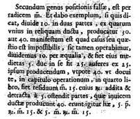
Cardano, Ars Magna, Chapter XXXVII (De regula falsum ponendi – the rule of a false proposition, a negative integer): “The second type of false solution lies in the root of a negative quantity (per radicem m). I will give an example. If someone demands to divide 10 into two parts, which when multiplied would equal 30 or 40, it is obvious that this case or question is impossible. But we will do as follows: we divide 10 in half, half will be 5; multiplied by itself, it comes to 25. Then deduct from 25 what should result from multiplication, say 40 – as I explained to you in the chapter on operations in the $4^{th}$ book; then we are left with $\sqrt{-15}$; if we deduct from this $\sqrt{-}$ and add to 5 or deduct from 5, then we get parts which when multiplied together give 40. Thus, these parts will be $5+\sqrt{-15}$ and $5-\sqrt{-15}$".
卡尔达诺，《大术》，第三十七章（关于假命题的规则 —— 负整数）：“第二种假解在于负数的根（通过 $\sqrt{-}$）。我举个例子。如果有人要求将 10 分成两部分，这两部分相乘等于 30 或 40，显然这个情况或问题是不可能的。但我们将这样做：我们将 10 分成两半，一半是 5；5 乘以 5 等于 25。然后从 25 中减去相乘应得的结果，比如 40 —— 正如我在第四本书的运算章节中向你解释的那样；然后我们得到 $\sqrt{-15}$ ；如果我们从这个数中减去或加上 5，或者从 5 中减去这个数，那么我们得到的两部分相乘等于 40。因此，这两部分将是 $5+\sqrt{-15}$ 和 $5-\sqrt{-15}$”

Here Cardano examines the equation $x(10-x)=40$, or $x^2+40=10x$ (the equation here should be written so that the coefficients are positive).
这里卡尔达诺研究的方程是 $x(10-x)=40$，即 $x^2+40=10x$（这里方程应写成系数为正的形式）。

Cardano solves this according to his rule, in modern notation: $x=5\pm \sqrt{25-40}=5\pm \sqrt{-15}$.
卡尔达诺按照他的规则求解，用现代符号表示为：$x=5\pm \sqrt{25-40}=5\pm \sqrt{-15}$。

The colon was used instead of a full stop.
冒号被用来代替句号。

Cardano shows that the derivation of the roots is 40.
卡尔达诺表明根的推导结果是 40。

In the text P means plus, and m means minus. R means radix, root; $5p:Rm:15$ means $5+\sqrt{-15}$; $5m:Rm:15$ signifies $5-\sqrt{-15}$; $25m:m:15$ quod est 40 signifies $25-(-15)=40$.
在文本中，P 表示加，m 表示减。R 表示 radix，即根；$5+\sqrt{-15}$ 表示为 $5p:Rm:15$；$5-\sqrt{-15}$ 表示为 $5m:Rm:15$；$25-(-15)=40$ 表示为 $25m:m:15$ quod est 40。

Cardano uses the fact that the complex roots when multiplied give a real number.
卡尔达诺利用了复数根相乘得到实数这一事实。

The history of the discovery of the formula for solving cubic equations is described in the books: Niccolò Tartaglia. Quesiti et inventioni diverse, dialogo con interlocutori principali Francesco Maria della Rovere e Gabriele Tadino e argomenti diversi: aritmetica, geometria, algebra, statica, topografia, artiglieria, fortificazioni, tattica. 1546.; Bortolotti, E. La storia della matematica nella Università di Bologna by Ettore Bortolotti. Bologna: N. Zanichelli, 1947. 226 p.; Guter R., Polunov Yu. Girolamo Kardano. M.: Znanie, 1980. 192 p. (Гутер Р., Полунов Ю. Джироламо Кардано. М.: Знание, 1980 г. 192 с.); S.G. Gindikin. Rasskazy o fizikah i matematikah (izdanie tret’e, rasshirennoe). M.: MCNMO, NMU, 2001. 448 p. (С.Г. Гиндикин. Рассказы о физиках и математиках (издание третье, расширенное). М.: МЦНМО, НМУ, 2001 г. 448 с.).
关于三次方程求解公式的发现历史，在以下书籍中有描述：尼科洛・塔尔塔利亚的《多样的问题与发明》；埃托雷・博尔托洛蒂的《博洛尼亚大学的数学史》；鲁道夫・古特尔和尤里・波卢诺夫的《杰罗拉莫・卡尔达诺》；S.G. 金迪金的《关于物理学家和数学家的故事》。

In 1572, a follower of Cardano, the hydraulic engineer Rafael Bombelli (1526–1572), wrote the book Algebra.

1572 年，卡尔达诺的追随者、水利工程师拉斐尔・邦贝利（1526 - 1572）撰写了《代数学》一书。

Where he first introduced the rules of arithmetic operations on negative numbers, and examined the solution of the cubic equations with roots of negative values.
在书中，他首次引入了负数的算术运算规则，并研究了带有负数根的三次方程的解法。

In solving these equations, where in auxiliary equations under the sign of the cubic radical it was possible to select the cube of the sum or the difference, and thus extract the cubic root, Bombelli showed that roots of negative values are mutually destroyed, as the components are mutually conjugate.
在求解这些方程时，在辅助方程的立方根符号下，可以选择和或差的立方，从而提取立方根。邦贝利表明，负数的根会相互抵消，因为这些分量是共轭的。

Bombelli showed the possibility of determining the ratio of equality, sum and derivation of complex numbers.
邦贝利展示了确定复数的相等、和与推导的比率的可能性。

But roots of negative values still had no physical or geometric meaning.
但负数的根仍然没有物理或几何意义。

Bombelli, as a hydraulic engineer, saw them as a useful auxiliary construction.
作为一名水利工程师，邦贝利将它们视为一种有用的辅助构造。

In 1637, René Descartes (1595–1650) published his Geometry, in which he called false roots “imaginary” (imaginariae).

1637 年，勒内・笛卡尔（1595 - 1650）出版了他的《几何学》，在书中他将假根称为 “虚数”（imaginariae）。

The term “real root” first appeared there.
“实根” 这个术语首次出现在那里。

He called negative roots false roots.
他把负根称为假根。

Descartes devised imaginary roots in solving the problem of crossing a circle with a parabola.
笛卡尔在解决圆与抛物线相交的问题时提出了虚根的概念。

Descartes examined cases of their intersection, touching, and the case “when the circle does not cross the parabola at any point, and this means that the equation does not have true or false roots, and that they are all imaginary”.
笛卡尔研究了它们相交、相切的情况，以及 “当圆与抛物线没有任何交点时，这意味着方程没有真根或假根，它们都是虚数” 的情况。

“There is no
value which corresponds to these imaginary roots”.
“没有任何值与这些虚根相对应”。

In 1685, John Wallis attempted to give a geometric and physical interpretation of negative and imaginary numbers.

1685 年 约翰・沃利斯的《代数学》

The first mathematician to attempt to give a geometric and physical interpretation of negative and imaginary numbers was John Wallis.
第一位试图对负数和虚数进行几何和物理解释的数学家是约翰・沃利斯。

This was in 1685, in his treatise Algebra.
这发生在 1685 年，在他的论文《代数学》中。

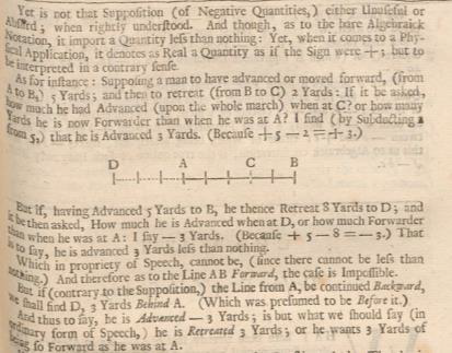
He explains negative numbers in a problem of displacement: “Yet is not that Supposition (of Negative Quantities,) either Unuseful or Absurd when rightly understood. And though, as to the bare Algebraick Notation, it import a Quantity less than nothing: Yet, when it comes to a Physical Application, it denotes as Real a Quantity as if the Sign were + but to be interpreted in a contrary sense.
他在一个位移问题中解释负数：“然而，对负数的这种假设（当正确理解时）既不是无用的，也不是荒谬的。虽然就纯粹的代数符号而言，它表示一个小于零的量；但当涉及到实际应用时，它表示的量与符号为 + 时一样真实，只是要从相反的意义上去解释。

As for instance: Supposing a man to have advanced or moved forward, (from A to B) 5 Yards; and then to retreat (from B to C ) 2 Yards: If he asked, how much he had Advanced (upon the whole march) when at $C?$ or how many Yards he is now Forwarder than when he was at A? I find (by Subducting 2 from 5,) that he is Advanced 3 Yards. (Because +5 –2=+3.)
例如：假设一个人向前行进或移动（从 A 到 B）5 码，然后向后撤退（从 B 到 C）2 码。如果问他在 C 点时总共前进了多少，或者他现在比在 A 点时向前了多少码？我通过从 5 中减去 2 得出，他前进了 3 码（因为 +5 – 2 = +3）。

But if, having Advanced 5 Yards to B , he thence Retreat 8 Yards to D ; and it be asked, How much he is Advanced when at D , or how much Forwarder than when he was at A : I say –3 Yards. ( Because $+5-8=-3$ ) That is to say, he is advanced 3 Yards left than nothing.
但是，如果他前进 5 码到达 B 点后，又从 B 点向后撤退 8 码到达 D 点，并且问他在 D 点时前进了多少，或者比在 A 点时向前了多少？我会说 -3 码。（因为 +5 – 8 = -3）也就是说，他比零前进了负 3 码。

Which in propriety of Speech, cannot be, (since there cannot be less than nothing.) And therefore as to the Line $AB$ Forward, the case is Impossible.
从严格意义上讲，这是不可能的（因为不可能有比零还少的情况）。因此，就向前的线段 AB 而言，这种情况是不可能的。

But if (contrary to the Supposition,) the Line from A , be continued Backward, we shall find D , 3 Yards behind A . (Which was presumed to be Before it.)
但是，如果（与假设相反）从 A 点开始的线段向后延伸，我们会发现 D 点在 A 点后方 3 码处（而之前假定它在 A 点前方）。

And thus to say, he is Advanced –3 Yards; is but what we should say (in ordinary form of Speech,) he is Retreated 3 Yards; or he wants 3 Yards of being so Forward as he was at $A^{\prime \prime \prime }$ You can see this text in the image below, the spelling and italics are original.
因此，说他前进了 -3 码，就相当于我们在日常表述中说他后退了 3 码，或者说他比在 A 点时少前进了 3 码。你可以从下面的图片中看到这段文字，拼写和斜体是原文的。

Imaginary numbers are like sides of a lost square field of earth10. An imaginary value for him is the “middle proportional value between a positive and negative value”. In his drawing we see that the imaginary number is a section of the $BP$ . This is Wallis’s argument:
虚数就像是一块丢失的正方形土地的边长。对他来说，虚数值是 “正数和负数之间的中间比例值”。在他的绘图中，我们可以看到虚数是线段 BP 的一部分。这是沃利斯的论证：

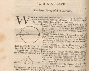
“What hath been already said of $\sqrt{-bc}$ in Algebra, (as I Mean Proportional between a Positive and a Negative Quantity:) may be thus Exemplified in Geometry.
“在代数学中关于 $\sqrt{-bc}$（作为正数和负数之间的中间比例）已经说过的内容，可以在几何学中这样举例说明。

For instance, if Forward from A , I take $AB=+b$ and Forward from thence, $BC=+c$ ; (making $AC=+AB+BC=+b+c$ , the Diameter of a Circle:) Then is the Sine11, or Mean Proportioned $BP=\sqrt{+bc}$ .
例如，如果从 A 点向前取 $AB=+b$，然后从 B 点再向前取 $BC=+c$（使得 $AC=+AB+BC=+b+c$，即圆的直径），那么正弦值或中间比例值 $BP=\sqrt{+bc}$。

But if Backward from A , I take $AB=-b$ ; and then Forward from that B , $BC=+c$ ; (making $AC=-AB+BC=-b+c$ ; the Diameter of the Circle:) Then is the Tangent or Mean Proportional $BP=\sqrt{-bc}$ .
但是，如果从 A 点向后取 $AB=-b$，然后从这个 B 点向前取 $BC=+c$（使得 $AC=-AB+BC=-b+c$，即圆的直径），那么正切值或中间比例值 $BP=\sqrt{-bc}$。

So that where $\sqrt{+bc}$ signifies a Sine; $\sqrt{-bc}$ shall signify a Tangent, to the same Arch (of the same Circle,) $AP$ , from the same point P , to the same Diameter $AC$
所以，当 $\sqrt{+bc}$ 表示正弦值时，$\sqrt{-bc}$ 将表示同一个圆中从同一点 P 到同一直径 AC 上同一弧 AP 的正切值。

Suppose now (for further Illustration,) A Triangle standing on the Line $AC$ (of indefinite length;) whose one Leg $AP=20$ is given; together with (the Angle $PAB$ , and consequently) the Height $PC=12$ ; and the length of the other Leg $PB=15$ : By which we are to find the length of the Base $AB$ .
现在进一步举例说明，假设有一个三角形，其底边为长度不确定的线段 AC，已知一条直角边 $AP=20$，以及（角 $PAB$，进而可知）高 $PC=12$，另一条直角边 $PB=15$。我们要据此求出底边 AB 的长度。

‘Tis manifest that the Square of $AP$ being 400; and of $PC$ , 144; their Difference 256 $(=400-144)$ is the Square of $AC$ .
显然，$AP$ 的平方是 400，$PC$ 的平方是 144，它们的差 256（ = 400 - 144）是 $AC$ 的平方。

And therefore $AC(=\sqrt{256})=+16$ , or –16; Forward or backward according as we please to take the Affirmative or Negative Root. But we will here take the Affirmative.
因此，$AC(=\sqrt{256})=+16$，或 -16，根据我们选择正根还是负根来确定向前或向后的方向。但在这里我们选择正根。

Then, because the Square of $PB$ is 225; and of $PC$ , 144; their Difference 81, is the Square of $CB$ . And therefore $CB=\sqrt{81}$ ; which is indifferently, +9 or –9; And may therefore be taken Forward or Backward from c . Which gives a Double value for the length of $AB$ ; to wit, $AB=16+9=25$ ;or $AB=16-9=7$ . Both Affirmative. (But if we should take, Backward from A , $AC=-16$ :then $AB=-16+9=-7$ ,and $AB=-16-9=-25$ . Both Negative.)
然后，因为 $PB$ 的平方是 225，$PC$ 的平方是 144，它们的差 81 是 $CB$ 的平方。因此，$CB=\sqrt{81}$，它可以是 +9 或 -9，可以从 C 点向前或向后取值。这就给 AB 的长度带来了两个值，即 $AB=16+9=25$ 或 $AB=16-9=7$，两个都是正值。（但如果我们从 A 点向后取 $AC=-16$，那么 $AB=-16+9=-7$，$AB=-16-9=-25$，两个都是负值。）

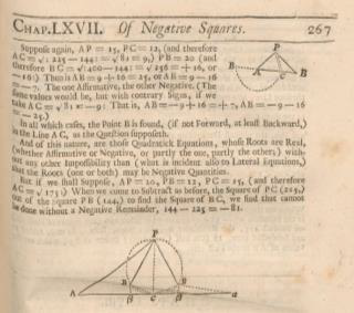
Suppose again, $AP=15$ , $PC=12$ ,(and therefore $AC=\sqrt{:225-144}:=\sqrt{81}=9,)PB=20$ (and therefore $BC=\sqrt{:400-144}:=\sqrt{256}=+16$ or –16:) Then is $AB=9+16=25$ ,or $AB=9-16=-7$ . The one Affirmative, the other Negative. (The same values would be, but with contrary Signs, if we take $AC=\sqrt{81}=-9$ : That is, $AB=-9+16=+7$ , $AB=-9-16=-25.$ )
再假设 $AP=15$，$PC=12$（因此 $AC=\sqrt{225-144}=\sqrt{81}=9$），$PB=20$（因此 $BC=\sqrt{400-144}=\sqrt{256}=+16$ 或 -16），那么 $AB=9+16=25$ 或 $AB=9-16=-7$，一个是正值，另一个是负值。（如果我们取 $AC=\sqrt{81}=-9$，那么会得到相同的值，但符号相反，即 $AB=-9+16=+7$，$AB=-9-16=-25$。）

In all which cases, the Point B is found, (if not Forward, at least Backward,) in the Line $AC$ , as the Question supposeth.
在所有这些情况下，根据问题的假设，点 B（如果不是在前方，至少在后方）都能在直线 AC 上找到。

And of this nature, are those Quadratick Equations, whose Roots are Real, (whether Affirmative or Negative, or partly the one, partly the other;) without any other Impossibility than (what is incident also to Lateral Equations,) that the Roots (one or both) may be Negative Quantities.
这类二次方程的根是实数（无论是正值、负值，还是部分为正部分为负），除了（与线性方程同样存在的）根（一个或两个）可能是负数之外，没有其他不可能的情况。

But if we shall Suppose, $AP=20$ , $PB=12$ , $PC=15$ ,(and therefore $AC=\sqrt{175}:$ ) When we come to Subtract as before, the Square of $PC$ (225,) out of the Square $PB$ (144,) to find the Square of $BC$ ,we find that cannot be done without a Negative Remainder, $144-225=-81$ .
但是，如果我们假设 $AP=20$，$PB=12$，$PC=15$（因此 $AC=\sqrt{175}$），当我们像之前那样计算，从 $PB$ 的平方（144）中减去 $PC$ 的平方（225）来求 $BC$ 的平方时，我们会发现无法得到非负的余数，144 - 225 = -81。

So that the Square of $BC$ is (indeed) the Difference of the Squares of $PB$ , $PC$ ; but a defective Deference; (that of $PC$ proving the greater, which was supposed the Lesser; and the Triangle $PBC$ , Rectangled, not as supposed at c , but at B ) And therefore $BC=\sqrt{-81}$ 1
所以，$BC$ 的平方确实是 $PB$ 和 $PC$ 平方的差，但这是一个不足的差（因为 $PC$ 的平方大于 $PB$ 的平方，而之前假设 $PB$ 的平方更大；并且三角形 $PBC$ 是直角三角形，但直角不是在 C 点，而是在 B 点）。因此，$BC=\sqrt{-81}$。

Which gives indeed (as before) a double value of $AB$ , $\sqrt{175}+\sqrt{-81}$ and $\sqrt{175},-\sqrt{-81}$ 顺事双 But such as requires a new Impossibility in Algebra, (which in Lateral Educations doth not happen;) not that of a Negative Root, or a Quantity less than nothing; (as before,) but the Root of a Negative Square. Which in strictness of speech, cannot be: since that no Real Root (Affirmative or Negative,) being Multiplied into itself, will make a Negative Square.
这确实（如之前一样）给 AB 带来了两个值，$\sqrt{175}+\sqrt{-81}$ 和 $\sqrt{175}-\sqrt{-81}$。但在代数学中，这需要一种新的不可能情况（这在线性方程中不会出现），不是负根或小于零的量（如之前那样），而是负数的平方根。严格来说，这是不可能的，因为任何实数根（无论是正数还是负数），自身相乘都不会得到负数的平方。

This Impossibility in Algebra, argues an Impossibility of the case proposed in Geometry; and that the Point B cannot be had, (as was supposed,) in the Line $AC$ , however produced (
forward or backward,) from A .
代数学中的这种不可能性表明，几何学中提出的情况也是不可能的，即点 B 无法在直线 AC 上（无论从 A 点向前还是向后延伸）找到。

Yet are there Two Points designed (out of that Line, but) in the same Plain; to either of which, if we draw the Lines $AB$ , $BP$ , we have a Triangle; whose Sides $AP$ , $PB$ are such as were required: And the Angle $PAC$ , and Altitude $PC$ , (above $AC$ , though not above $AB$ ,) such as proposed; And the Difference of Squares of $PB$ $PC$ , is that of $CB$
然而，在同一平面上（不在直线 AC 上）存在两个点，从 A 点向这两个点中的任意一个点绘制线段 AB 和 BP，都能构成一个三角形，其边 AP 和 PB 满足要求，角 $PAC$ 和高于 $AC$（尽管不是高于 AB）的高 $PC$ 也符合提议，并且 $PB$ 和 $PC$ 平方的差就是 $CB$ 的平方。

And like as in the first case, the Two values of $AB$ (which are both Affirmative,) make the double of AC, $(16+9,+16-9,=16+16=32:$ So here, $\sqrt{175}+\sqrt{-81}+\sqrt{175}-\sqrt{-81}=2\sqrt{175}$
就像在第一种情况下，AB 的两个正值（16 + 9 和 +16 - 9）使得 AC 的长度加倍（16 + 16 = 32）一样，在这里，$\sqrt{175}+\sqrt{-81}+\sqrt{175}-\sqrt{-81}=2\sqrt{175}$。

And (in the Figure,) though not the Two Lines themselves, $AB$ , $AB$ , (as in the First case, where they lay in the Line $AC;$ ) yet the Ground-lines on which they stand, $A\beta$ , $A\beta$ β, are Equal to the Double of $AC$ : That is, if to either of those $AB$ , we join $B\alpha$ α, equal to the other of them, and with the same Declivity; $AC\alpha$ α (the Distance of $A\alpha$ α) will be a Streight Line equal to the double of $AC$ ; as is ACα in the First case.
（在图中）尽管不像第一种情况那样，两条线段 AB 本身（它们位于直线 AC 上），但它们所在的基线 $A\beta$ 和 $A\beta$β 等于 AC 长度的两倍。也就是说，如果我们将其中一条 AB 与等于另一条 AB 的 $B\alpha$α 连接起来，并且具有相同的倾斜度，那么 $AC\alpha$α（$A\alpha$α 之间的距离）将是一条与 AC 长度两倍相等的直线，就像第一种情况中的 ACα 一样。

But in both $AC\alpha$ (the Ground - Lines of $AB\alpha$) is Equal to the Double of $AC$.
但在两种情况下，$AC\alpha$（$AB\alpha$ 的基线）都等于 $AC$ 的两倍。

So that, whereas in case of Negative Roots, we are to say, The Point $B$ cannot be found, so as is supposed in $AC$ Forwards, but Backwards from $A$ it may in the same Line: We must here say, case of a Negative Square, the Point $B$ cannot be found so as was supposed, in the Line $AC$ but Above that Line it may in the same Plain.
所以，在负根的情况下，我们不得不说，点 $B$ 无法在 $AC$ 向前的方向上找到，但可以在从 $A$ 向后的同一条直线上找到；而在这里，对于负数平方的根这种情况，我们必须说，点 $B$ 无法在直线 $AC$ 上找到，但可以在该直线上方的同一平面内找到。

Unfortunately, Wallis’s suggestion that complex number were not located on a straight lane, but on a complex plane, was incomprehensible to his contemporaries.
不幸的是，沃利斯关于复数不是位于直线上，而是位于复平面上的观点，在当时无法被他的同时代人理解。

For a number to become a mathematical object, its ratios had to be determined (equality, less, more, i.e. order) and operations on objects.
要使一个数成为数学对象，就必须确定它的各种关系（相等、小于、大于，即顺序）以及对这些对象的运算。

But it was unclear whether an operation on complex numbers would always lead to a number of this kind, i.e. $x+y\sqrt{-1}$.
但当时还不清楚对复数进行运算是否总能得到这种形式的数，即 $x+y\sqrt{-1}$。

In 1702, Gottfried Wilhelm Leibniz tried to prove this, but failed.

1702 年，莱布尼茨

Gottfried Wilhelm Leibniz tried to prove this in 1702, but failed.
戈特弗里德・威廉・莱布尼茨在 1702 年试图证明这一点，但失败了。

In the article Graphic proof of the new analysis for recognizing infinity in relation to sums and quadratics, breaking down the binomial into multiples, Leibniz arrived at the result $x^4+a^4=(x+a\sqrt{\sqrt{-1}})(x-a\sqrt{\sqrt{-1}})(x+a\sqrt{-\sqrt{-1}})(x-a\sqrt{-\sqrt{-1}})$, and concluded that an imaginary number of a different kind existed.
在《关于无穷级数和二次型的新分析的图形证明》一文中，莱布尼茨将二项式分解为多个因式，得到结果 $x^4+a^4=(x+a\sqrt{\sqrt{-1}})(x-a\sqrt{\sqrt{-1}})(x+a\sqrt{-\sqrt{-1}})(x-a\sqrt{-\sqrt{-1}})$，并得出存在不同类型虚数的结论。

He called imaginary numbers idealis mundi monstro: “Itaque elegans et mirabile effugium repetir in illo Analyseos miraculo, idealis mundi monstro, pene inter Ens et non - Ens Amphibio, quod radicem imaginariam appellamus”. – “What we call the imaginary root is an elegant and wonderful invention in this incredible analysis, the prototype of a monster of the world, an amphibian between being and non - being”.
他将虚数称为 “理想世界的怪物”：“因此，在这令人难以置信的分析中，我们找到了一个优雅而奇妙的方法，那就是我们所称的虚根，它是理想世界的怪物，几乎是存在与非存在之间的两栖物。”

In 1702, Johann Bernoulli encountered the problem of calculating the logarithm of a complex number.

1712 年 负数和虚数的对数

Before 1702, imaginary numbers were only seen as roots of negative values.
在 1702 年之前，虚数仅被视为负数的根。

In 1702, Johann Bernoulli encountered the problem of calculating the logarithm of a complex number.
1702 年，约翰・伯努利遇到了计算复数对数的问题。

By 1712, Bernoulli and Leibniz had argued about what the logarithm of a negative number was.
到 1712 年，伯努利和莱布尼茨就负数的对数展开了争论。

For the positive number $a$, it was fair to state $\ln \sqrt{a}=\frac{1}{2}\ln a$.
对于正数 $a$，可以合理地说 $\ln \sqrt{a}=\frac{1}{2}\ln a$。

Continuing the argument, it may be concluded that $\ln i=\ln \sqrt{-1}=\frac{1}{2}\ln (-1)$.
继续推理，可以得出 $\ln i=\ln \sqrt{-1}=\frac{1}{2}\ln (-1)$。

But what is equal to $\ln (-1)$?
但是 $\ln (-1)$ 等于什么呢？

Leibniz believed that it must be complex.
莱布尼茨认为它一定是复数。

Bernoulli, and d’Alembert after him, believed that it was substantial.
伯努利以及之后的达朗贝尔则认为它是实数。

The English mathematician and astronomer R. Cotes, in his work Logometria, 1714, published in Philosophical Transactions in 1717, placed the formula $\ln (\cos x+i\sin x)=xi$, expressed in the following words: “If any arc of a quarter of a circle, described by the radius, $CE$, has the sine $SX$ and the cosine to the quarter $XE$ and if the radius $CE$ is taken for the module, then the arc will be the measure of the ratio $\frac{EX+XC\sqrt{-1}}{CE}$, multiplied by $\sqrt{-1}$”.
英国数学家和天文学家 R. 科茨在他 1714 年的著作《对数计算》（1717 年发表于《哲学汇刊》）中提出公式 $\ln (\cos x+i\sin x)=xi$，用以下文字表述：“如果以半径 $CE$ 描述的四分之一圆的任何弧，其正弦为 $SX$，余弦为 $XE$，并且以半径 $CE$ 为模，那么该弧将是 $\frac{EX+XC\sqrt{-1}}{CE}$ 的比值的度量，再乘以 $\sqrt{-1}$”。

Cotes did not give any applications for this.
科茨没有给出这个公式的任何应用。

In 1749 Euler proved it, confirming that Leibniz was correct.
1749 年，欧拉证明了这个公式，证实莱布尼茨是正确的。

Now we know this formula as $\text{Ln}z=\ln |z|+i\phi +2k\pi i$.
现在我们知道这个公式为 $\text{Ln}z=\ln |z|+i\phi +2k\pi i$。

In 1707, and later in 1722, Abraham de Moivre made a trigonometric interpretation of the complex number.

1707 年和 1722 年。亚伯拉罕・棣莫弗的三角表示法

In 1707, and later in 1722, Abraham de Moivre made a trigonometric interpretation of the complex number.
1707 年，以及后来在 1722 年，亚伯拉罕・棣莫弗对复数进行了三角解释。

Cubic equations and higher were solved not only by the algebraic method, but also by the trigonometric method, using the sinus of short arcs.
三次及更高次方程不仅可以用代数方法求解，还可以用三角方法，利用短弧的正弦来求解。

In 1594, Francois Viète had solved an equation of the $45^{th}$ degree using this method.
1594 年，弗朗索瓦・韦达就曾用这种方法解出了一个 45 次方程。

Moivre reached a formula of raising the degree and extracting the root of a natural degree (up to the $7^{th}$) of a complex number.
棣莫弗利用已知的关系，得出了复数的幂次提升和自然数次方根提取（最高到 7 次）的公式。

It is interesting that he examined the circular arc $x^2+y^2=1$, and then the hyperbolic arc $x^2-y^2=1$, which led him to the idea of the imaginary substituting $y=v\sqrt{-1}$.
有趣的是，他研究了单位圆 $x^2+y^2=1$，然后研究了双曲线弧 $x^2-y^2=1$，这使他产生了用 $y=v\sqrt{-1}$ 进行虚数代换的想法。

But even when he presented a complex number in trigonometric form, Moivre did not depict it on a surface.
但即使他将复数表示为三角形式，棣莫弗也没有将其描绘在平面上。

In Petersburg in the 1730s–1740s, Leonhard Euler developed the rudiments of the theory of functions of the complex variable.

莱昂哈德・欧拉

In Petersburg in the 1730s–1740s, Leonhard Euler developed the rudiments of the theory of functions of the complex variable.
在 18 世纪 30 - 40 年代的圣彼得堡，莱昂哈德・欧拉发展了复变函数理论的雏形。

In his works, Euler moved from coordinates of a point $(x,y)$ to the complex number $p=x\pm \sqrt{-1}y$, and represented it in the polar coordinates $p=s(\cos \omega \pm \sqrt{-1}\sin \omega )$.
在他的著作中，欧拉从点 $(x,y)$ 的坐标转换到复数 $p=x\pm \sqrt{-1}y$，并将其表示为极坐标形式 $p=s(\cos \omega \pm \sqrt{-1}\sin \omega )$。

This concept was used after Euler by Lagrange and other mathematics in two - dimensional problems of mathematical physics, but at that time there was no geometric, let alone physical concept of operations on complex numbers.
欧拉之后，拉格朗日和其他数学家在数学物理的二维问题中使用了这个概念，但在当时，对于复数的运算还没有几何意义，更不用说物理意义了。

In 1743, Euler created the method of solving linear differential equations of higher orders, in which in solving characteristic algebraic equations, imaginary numbers arise.
1743 年，欧拉创立了求解高阶线性微分方程的方法，在求解特征代数方程时会出现虚数。

At the same time, the general solution of the equation is valid.
与此同时，该方程的通解是有效的。

In 1748, Euler proved Moivre’s formula for all valid $n$.
1748 年，欧拉证明了棣莫弗公式对所有有效 $n$ 都成立。

Now it is proven as a consequence from Euler’s formula $e^{i\phi }=\cos \phi +i\sin \phi$.
现在，它是作为欧拉公式 $e^{i\phi }=\cos \phi +i\sin \phi$ 的推论被证明的。

Euler published this formula in an article of 1740 and in the $7^{th}$ chapter of his book Introduction to an analysis of infinitesimals (Introductio in analysin infinitorum, 1748 г.).
欧拉在 1740 年的一篇文章和他 1748 年的著作《无穷小分析引论》（Introductio in analysin infinitorum）的第 7 章中发表了这个公式。

Euler gradually gained an understanding of the concept of the complex number.
欧拉逐渐理解了复数的概念。

He made a large number of observations of his own mathematical studies, but not all of them found a geometric or physical interpretation.
他在自己的数学研究中进行了大量观察，但并非总
能找到几何或物理解释。

A.I. Markushevich noted this fact.
A. I. 马尔库舍维奇注意到了这一事实。

In 1741 Euler in a letter to Goldbach (9.XII. 1741) wrote: “I recently found a wonderful paradox, that this value of the expression $\frac{2^{+\sqrt{-1}}+2^{-\sqrt{-1}}}{2}$ is very close to $\frac{10}{13}$ o a The true value of this expression is the cosine of the arc … 9 9 5 5 0 8 1 7 4 1 3 9 6 ,0 ”.
1741 年，欧拉在给哥德巴赫的一封信（1741 年 12 月 9 日）中写道：“我最近发现了一个奇妙的悖论，表达式 $\frac{2^{+\sqrt{-1}}+2^{-\sqrt{-1}}}{2}$ 的值非常接近 $\frac{10}{13}$。这个表达式的真实值是某段弧的余弦值……”

The meaning of this statement becomes clear if we represent $\frac{2^{+\sqrt{-1}}+2^{-\sqrt{-1}}}{2}$ in the form $\frac{e^{+\sqrt{-1}\ln 2}+e^{-\sqrt{-1}\ln 2}}{2}$, which according to Euler’s formula from “An introduction to an analysis of infinitesimals”, $ \cos v=\frac {e^{+v\sqrt {-1}}+e^{-v\sqrt {-1}}}{2}$ gives $\cos (\ln 2)$.
如果我们将 $\frac{2^{+\sqrt{-1}}+2^{-\sqrt{-1}}}{2}$ 表示为 $\frac{e^{+\sqrt{-1}\ln 2}+e^{-\sqrt{-1}\ln 2}}{2}$，根据欧拉《无穷小分析引论》中的公式 $\cos v=\frac{e^{+v\sqrt{-1}}+e^{-v\sqrt{-1}}}{2}$，就可以得到 $\cos (\ln 2)$。

Euler gave the value of $\ln 2$.
欧拉给出了 $\ln 2$ 的值。

In his article Studies on imaginary roots of equations (Recherches sur les racines imaginaires des équations. Mém. Ac. Berlin, (1749) 1751) examined the issue of the possible form of a complex number.

1749/51 年，欧拉

In his article Studies on imaginary roots of equations (Recherches sur les racines imaginaires des équations. Mém. Ac. Berlin, (1749) 1751) Euler examined the issue of the possible form of a complex number.
在他的文章《关于方程虚根的研究》（Recherches sur les racines imaginaires des équations. Mém. Ac. Berlin, (1749) 1751）中，欧拉研究了复数可能的形式问题。

“A quantity is named imaginary is it is not greater than zero, not less than zero or equal to zero; this, accordingly, is something impossible, for example $\sqrt{-1}$, or even $a+b\sqrt{-1}$, as this quantity is not positive, or negative, or zero”.
“A quantity is named imaginary is it is not greater than zero, not less than zero or equal to zero; this, accordingly, is something impossible, for example $\sqrt{-1}$, or even $a+b\sqrt{-1}$, as this quantity is not positive, or negative, or zero”。

Euler examines the main theorem of algebra that he has proven as a separate case of the following proposal “any imaginary quantity is always formed by two members, one of which is a real quantity indicated by $M$, and the other is a derivate of this real quantity $N$ by $\sqrt{-1}$; thus $\sqrt{-1}$, is the only source of all imaginary expressions”.
欧拉研究了他所证明的代数基本定理，将其作为以下命题的一个特殊情况：“任何虚数总是由两部分组成，其中一部分是实数，用 $M$ 表示，另一部分是这个实数 $N$ 与 $\sqrt{-1}$ 的乘积；因此，$\sqrt{-1}$ 是所有虚数表达式的唯一来源”。

For proof, Euler applied to numbers of the type $a+b\sqrt{-1}$ various algebraic and transcendental operations which were known in his time, and showed that the result would be a number of the same kind.
为了证明这一点，欧拉对 $a+b\sqrt{-1}$ 这种类型的数应用了当时已知的各种代数和超越运算，并表明结果仍然是同一种类型的数。

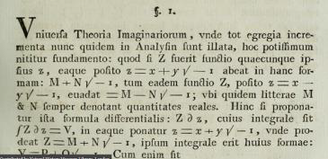
In 1752, d’Alembert examined the perfect fluid motion.

1752 年。让・勒朗・达朗贝尔。柯西 - 黎曼方程

In the $18^{th}$ century, hydrodynamics developed swiftly.
在 18 世纪，流体动力学迅速发展。

In 1752, d’Alembert examined the perfect fluid motion.
1752 年，达朗贝尔研究了理想流体的运动。

In the article Essai d’une nouvelle théorie de la résistance des fluides, d’Alembert determined the speed $f(x,y)=u(x,y)+v(x,y)\sqrt{-1}$, where the functions $u(x,y)$ and $v(x,y)$ are projections of the speed of a particle of liquid on the axis of coordinates. They are connected by the equations $\frac{\partial v}{\partial x}=-\frac{\partial u}{\partial y}$ and $\frac{\partial u}{\partial x}=\frac{\partial v}{\partial y}$ (with the differential forms $v\mathrm{d}x+u\mathrm{d}y$ and $u\mathrm{d}v-v\mathrm{d}y$, and the compact notation $\frac{\partial f}{\partial x}+i\frac{\partial f}{\partial y}=0$).
在《关于流体阻力的新理论的尝试》一文中，达朗贝尔确定了速度 $f(x,y)=u(x,y)+v(x,y)\sqrt{-1}$，其中函数 $u(x,y)$ 和 $v(x,y)$ 是液体粒子在坐标轴上的速度投影。它们由方程 $\frac{\partial v}{\partial x}=-\frac{\partial u}{\partial y}$ 和 $\frac{\partial u}{\partial x}=\frac{\partial v}{\partial y}$（用微分形式表示为 $v\mathrm{d}x+u\mathrm{d}y$ 和 $u\mathrm{d}v-v\mathrm{d}y$，紧凑记法为 $\frac{\partial f}{\partial x}+i\frac{\partial f}{\partial y}=0$ ）相联系。

In 1755, Euler arrived at the same results, and later established that the actual and imaginary part of any analytical function necessarily satisfy these conditions:
1755 年，欧拉得出了相同的结果，随后他确定任何解析函数的实部和虚部必然满足这些条件：

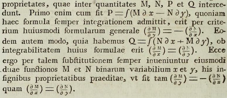
(Figure 5, Euler L. Ulterior disquisitio de formulis integralibus imaginariis. Properties that exist between quantities $M$, $N$, $P$ and $Q$. Firstly, since $P=\int (M\partial x-N\partial y)$, because this formula always admits integration, according to the general criterion of such formulas $(\frac{\partial \underline{H}}{\partial y})=-(\frac{\partial \underline{\partial }}{\partial x})$. Similarly, since we have $Q=\int (N\partial x+M\partial y)$, due to the integrability of this formula, there will be $(\frac{\partial E}{\partial x})=(\frac{\partial b}{\partial y})$. Thus, through such a substitution, two functions $M$ and $N$ of the variables $r$ and $y$ can always be found, which have these remarkable properties, such that $(\frac{\partial u}{dy})÷-(\frac{\partial x}{dx})$ and $(\frac{\partial y}{\partial x})=(\frac{\partial x}{\partial y})$.)
（图 5，欧拉《关于虚积分公式的进一步研究》，在量 $M$、$N$、$P$ 和 $Q$ 之间存在的性质。首先，由于 $P=\int (M\partial x-N\partial y)$，因为这个公式总是可以积分，根据这类公式的一般准则 $(\frac{\partial \underline{H}}{\partial y})=-(\frac{\partial \underline{\partial }}{\partial x})$。同样地，因为我们有 $Q=\int (N\partial x+M\partial y)$，由于这个公式的可积性，将有 $(\frac{\partial E}{\partial x})=(\frac{\partial b}{\partial y})$。因此，通过这样的代换，总是可以找到两个关于变量 $r$ 和 $y$ 的函数 $M$ 和 $N$，它们具有这些显著的性质，使得 $(\frac{\partial u}{dy})÷-(\frac{\partial x}{dx})$ 以及 $(\frac{\partial y}{\partial x})=(\frac{\partial x}{\partial y})$ 。）

Euler’s works set out the theory of elementary functions of a complex variable. Today, these are called Cauchy–Riemann conditions, and are the conditions for the analysis of a function. For this function the family of curves $u(x,y)=C$ and $v(x,y)=C$ are mutually orthogonal.
欧拉的工作阐述了复变初等函数的理论。如今，这些条件被称为柯西 - 黎曼条件，是函数可解析的条件。对于这样的函数，曲线族 $u(x,y)=C$ 和 $v(x,y)=C$ 相互正交。

In the Universal Arithmetic of 1768 in Russian, Euler writes “Roots from negative numbers are not more or less than nothing, and they are also not nothing, for $0$ multiplied by $0$ in derivation gives $0$, and accordingly is not a negative number.

1768 年欧拉《通用算术》

Operations of deriving the root continued to present difficulties for a long time. In the Universal Arithmetic of 1768 in Russian, Euler writes “Roots from negative numbers are not more or less than nothing, and they are also not nothing, for $0$ multiplied by $0$ in derivation gives $0$, and accordingly is not a negative number.
求根运算在很长一段时间内都存在困难。1768 年，欧拉在俄文版的《通用算术》中写道：“负数的根既不大于零，也不小于零，也不等于零，因为 $0$ 乘以 $0$ 在求根时得到 $0$，因此它不是负数。

When all possible numbers which can be imagined are more or less than $0$ or $0$ itself, it can be seen that the square roots of negative numbers cannot be included in the group of possible numbers, and accordingly they are impossible numbers. This fact leads us to a recognition of these numbers, which by their property are impossible and are usually called imaginary numbers, because they can only be imagined in the mind.” (Euler’s italics)
当所有可以想象的数要么大于 $0$，要么小于 $0$，要么等于 $0$ 时，可以看出负数的平方根不能被归入可能的数的范畴，因此它们是不可能的数。这一事实使我们认识到这些数，由于其性质是不可能的，通常被称为虚数，因为它们只能在头脑中想象。”（欧拉原文斜体强调）

But Euler goes on to make a mistaken argument: “But when $\sqrt{a}$, multiplied by $\sqrt{b}$, gives $\sqrt{ab}$; then $\sqrt{-2}$, multiplied by $\sqrt{-3}$, will give $\sqrt{6}$; equally $\sqrt{-1}$, multiplied by $\sqrt{-4}$, will give $\sqrt{4}$, i.e. $2$; from this we can see that two impossible numbers multiplied together we can get a possible or real number. But when $\sqrt{-3}$ is multiplied by $\sqrt{+5}$, we get $\sqrt{-15}$, or a possible number, multiplied by an impossible one always give an impossible number”.
但欧拉接着提出了一个错误的论证：“但是当 $\sqrt{a}$ 乘以 $\sqrt{b}$ 得到 $\sqrt{ab}$ 时，那么 $\sqrt{-2}$ 乘以 $\sqrt{-3}$ 将得到 $\sqrt{6}$；同样，$\sqrt{-1}$ 乘以 $\sqrt{-4}$ 将得到 $\sqrt{4}$，即 $2$；由此我们可以看到，两个不可能的数相乘可以得到一个可能的或实数。但是当 $\sqrt{-3}$ 乘以 $\sqrt{+5}$ 时，我们得到 $\sqrt{-15}$，也就是说，一个可能的数乘以一个不可能的数总是得到一个不可能的数。”

As we can see, operations on complex numbers were not yet clear, but 9 years later Euler corrected his error, defining $\sqrt{-1}$ as the imaginary $i$, the square of which is equal to $-1$, i.e. $\frac{1}{i}=-i$.
正如我们所见，当时对复数的运算还不清晰，但 9 年后欧拉纠正了他的错误，将 $\sqrt{-1}$ 定义为虚数 $i$，其平方等于 $-1$，即 $\frac{1}{i}=-i$。

Euler discussed the issue on the expedience of imaginary numbers: “It finally remains to dispel the doubt about when these forces are impossible, it seems that they are completely unnecessary, and this science may be considered worthless. But despite this, it is in fact very necessary, for such issues often arise, in which we cannot discover swiftly whether they are possible or impossible. But when their solution brings us to these impossible numbers, this will mean that the actual issue is impossible. To clarify this with an example, let us examine the following issue: the number $12$ divided into two parts, the product of which would be $40$. When we solve this issue in the next rules, we will find for the two numbers $6+\sqrt{-4}$ and $6-\sqrt{-4}$, which accordingly are impossible: thus, from this we see that this problem cannot be solved… If the number $12$ must be divided into two such parts, which would give $35$, then these parts would undoubtedly be $7$ and $5$”.
欧拉讨论了虚数的实用性问题：“最后，关于这些虚数在何种情况下是不必要的疑虑依然存在，似乎它们完全没有必要，相关科学也可能被认为毫无价值。但尽管如此，实际上它们非常必要，因为经常会出现这样的问题，我们无法迅速判断它们是否可行。但是当它们的解使我们得到这些不可能的数时，这将意味着实际问题是不可能解决的。为了用一个例子说明这一点，让我们考虑以下问题：将 $12$ 分成两部分，它们的乘积为 $40$。当我们按照通常的规则解决这个问题时，我们会得到两个数 $6+\sqrt{-4}$ 和 $6-\sqrt{-4}$，因此它们是不可能的；由此我们可以看出这个问题无法解决。如果要将 $12$ 分成两部分，使其乘积为 $35$，那么这两部分无疑是 $7$ 和 $5$。”

In the paper On forms of differentials of angles, especially with irrationalities, which are integrated with the assistance of logarithms and circular arcs, Master of natural sciences of the Academy presented on 5 May 1777, published in 1794, for the first time Euler introduced the symbol of the imaginary unit $i$, from the first letter of imaginaire, which is what Descartes called imaginary numbers.

1777 年，欧拉引入符号 $i$

In the paper On forms of differentials of angles, especially with irrationalities, which are integrated with the assistance of logarithms and circular arcs, Master of natural sciences of the Academy presented on 5 May 1777, published in 1794, for the first time Euler introduced the symbol of the imaginary unit $i$, from the first letter of imaginaire, which is what Descartes called imaginary numbers.
在 1777 年 5 月 5 日提交、1794 年发表的《关于角度微分形式，特别是借助对数和圆弧进行积分的无理形式》一文中，科学院的自然科学硕士欧拉首次引入了虚数单位 $i$ 的符号，它取自笛卡尔对虚数的称呼 “imaginaire” 的首字母。

(Figure 6. The first appearance of symbol “$i$”)
（图 6. 符号 “$i$” 的首次出现）

Translation: We will examine and study the differential formula $\frac{\partial \Phi \cos \Phi }{\sqrt[n]{\cos .n\Phi }}$, the integral of the logarithm of the circular arcs. Solution. For this I believe another method is also available, which however requires the imaginary unit $\sqrt{-1}$, which in future we will designate by the letter $i$, $i^2=-1$, or $\frac{1}{i}=-i$. Above all, we note that the value of our formula, $\cos \Phi$ can be replaced by two parts $\partial p=\frac{\partial \Phi (\cos .\Phi +i\sin .\Phi )}{\sqrt[n]{\cos .n\Phi }}$ and $\partial q=\frac{\partial \Phi (\cos .\Phi -i\sin .\Phi )}{\sqrt[n]{\cos n\Phi }}$, and then our formula may be represented as $\frac{1}{2}\partial p+\frac{1}{2}\partial q$, and the integral is expressed as $\frac{p+q}{2}$.
译文：我们将研究和探讨微分公式 $\frac{\partial \Phi \cos \Phi }{\sqrt[n]{\cos .n\Phi }}$，它是对数和圆弧积分的公式。解决方案。我认为还有另一种方法，然而这种方法需要虚数单位 $\sqrt{-1}$，在今后我们将用字母 $i$ 来表示它，$i^2=-1$，或者 $\frac{1}{i}=-i$。首先，我们注意到我们公式中的 $\cos \Phi$ 的值可以被分成两部分 $\partial p=\frac{\partial \Phi (\cos .\Phi +i\sin .\Phi )}{\sqrt[n]{\cos .n\Phi }}$ 和 $\partial q=\frac{\partial \Phi (\cos .\Phi -i\sin .\Phi )}{\sqrt[n]{\cos n\Phi }}$，然后我们的公式可以表示为 $\frac{1}{2}\partial p+\frac{1}{2}\partial q$，其积分表示为 $\frac{p+q}{2}$。

In the 1770s, Euler’s changed his attitude towards imaginary numbers. From auxiliary formalism, it acquired the necessary theoretical status, receiving the definition ($i^2=-1$) and a description of properties.
在 18 世纪 70 年代，欧拉对虚数的态度发生了变化。虚数从辅助形式主义转变为具有必要理论地位的概念，得到了定义（$i^2=-1$）并对其性质进行了描述。

Euler developed the theory of integrals of the function of the complex variable, and also singled out the principle of symmetry. “The entire theory of imaginary numbers, to which analysis is now obliged for so much success, rests primarily on the following foundation: if $Z$ is any function from $z$, which after the substitution $z=x+y\sqrt{-1}$ takes the following form: $M+N\sqrt{-1}$, which by the substitution $z=x-y\sqrt{-1}$ the same function $M-N\sqrt{-1}$, where the letters $M$ and $N$ always mean real quantitates”.
欧拉发展了复变函数积分理论，还提出了对称原理。“整个虚数理论，如今分析学取得的诸多成功都归功于它，主要基于以下基础：如果 $Z$ 是关于 $z$ 的任意函数，在 $z=x+y\sqrt{-1}$ 的代换下，它具有 $M+N\sqrt{-1}$ 的形式，而在 $z=x-y\sqrt{-1}$ 的代换下，同一个函数变为 $M-N\sqrt{-1}$，其中字母 $M$ 和 $N$ 始终表示实数。”

From this, the Euler–d’Alembert formulas follow, or as we call them today, the Cauchy–Riemann formulas.
由此得出欧拉 - 达朗贝尔公式，也就是我们如今所说的柯西 - 黎曼公式。

(Figure 7. Euler on the symmetry property)
（图 7. 欧拉关于对称性质）

Euler then applied the function of the complex variable to conformal transformations (preserving the angles and likeness in the small).
随后，欧拉将复变函数应用于保角变换（在小范围内保持角度和相似性）。

The geometric interpretation of complex numbers and operations with them was first given by the Norwegian geodesist and cartographer of the Danish academy of sciences Caspar Wessel (1745–1818) in the work An essay on the analytical representation of direction and its applications, primarily to the solution of flat and spherical polygons, submitted in 1797 and published in Danish in 1799. He wrote the work for cartographers.

1797/1799 年，卡斯帕・韦塞尔

The geometric interpretation of complex numbers and operations with them was first given by the Norwegian geodesist and cartographer of the Danish academy of sciences Caspar Wessel (1745–1818) in the work An essay on the analytical representation of direction and its applications, primarily to the solution of flat and spherical polygons, submitted in 1797 and published in Danish in 1799. He wrote the work for cartographers.
复数及其运算的几何解释最早由丹麦科学院的挪威测量员和制图师卡斯帕・韦塞尔（1745 - 1818）在《关于方向的解析表示及其应用，主要用于平面和球面多边形的求解》一文中给出，该文于 1797 年提交，1799 年以丹麦语发表。他撰写这篇文章是为了制图师。

Wessel introduced the concept of the directed section, and defined structure as the parallel displacement of a plane, and multiplication as the rotation of a plane with expansion.
韦塞尔引入了有向线段的概念，将结构定义为平面的平行位移，将乘法定义为平面的旋转和拉伸。

In his work, Wessel writes: “Let +1 indicate a positive linear unit, and $\epsilon$ another different unit perpendicular to the positive unit and having the same origin. Then the directing angle +1 will be equal to $0^{\circ }$, for –1 will be equal to $180^{\circ }$, for $\epsilon$ will be equal to $90^{\circ }$, for $-\epsilon$ will be equal to $-90^{\circ }$ or $270^{\circ }$. Owing to the rule that the directing angle of product is equal to the sum of the angle of co - multipliers, we will obtain: $(+1)(+1)=+1$, $(+1)(-1)=-1$, $(-1)(-1)=+1$, $(+1)(+\epsilon )=+\epsilon$, $(+1)(-\epsilon )=-\epsilon$, $(-1)(+\epsilon )=-\epsilon$, $(-1)(-\epsilon )=+\epsilon$, $(+\epsilon )(+\epsilon )=-1$, $(+\epsilon )(-\epsilon )=+1$, $(-\epsilon )(-\epsilon )=-1$. From this it is clear that $\epsilon$ is equivalent to $\sqrt{-1}$, and the deviation of the product is determined in such a way that not one of the general rules violates this operation”.
在他的作品中，韦塞尔写道：“令 $+1$ 表示正线性单位，$\epsilon$ 表示与正单位垂直且原点相同的另一个不同单位。那么 $+1$ 的方向角将等于 $0^{\circ }$，$-1$ 的方向角等于 $180^{\circ }$，$\epsilon$ 的方向角等于 $90^{\circ }$，$-\epsilon$ 的方向角等于 $-90^{\circ }$ 或 $270^{\circ }$。根据乘积的方向角等于各乘数方向角之和的规则，我们将得到：$(+1)(+1)=+1$，$(+1)(-1)=-1$，$(-1)(-1)=+1$，$(+1)(+\epsilon )=+\epsilon$，$(+1)(-\epsilon )=-\epsilon$，$(-1)(+\epsilon )=-\epsilon$，$(-1)(-\epsilon )=+\epsilon$，$(+\epsilon )(+\epsilon )=-1$，$(+\epsilon )(-\epsilon )=+1$，$(-\epsilon )(-\epsilon )=-1$。由此可见，$\epsilon$ 等同于 $\sqrt{-1}$，并且乘积的偏差是以这样一种方式确定的，即没有任何一般规则会违反这种运算。”

Wessel showed that complex numbers represented by directed segments obey non - contradictory arithmetic. The sum of the two complex numbers $a+bi$ and $c+di$ Wessel calls the diagonal of a parallelogram, built on the sides of directed segments, corresponding to the components, i.e. parallel displacement of the plane along $a+bi$.
韦塞尔表明，用有向线段表示的复数遵循无矛盾的算术规则。两个复数 $a+bi$ 和 $c+di$ 的和，韦塞尔称之为以对应于这两个复数的有向线段为边构建的平行四边形的对角线，即平面沿着 $a+bi$ 的平行位移。

Multiplication of the two complex numbers $(a+bi)(c+di)=(a+bi)\rho e^{i\phi }$ (where $\rho e^{i\phi }=c+di$) reflects the rotation of plane around the point $o$ to the angle $\phi$ with the extension of all segments in the relation of $\rho$.
两个复数 $(a+bi)(c+di)=(a+bi)\rho e^{i\phi }$（其中 $\rho e^{i\phi }=c+di$）的乘法反映了平面绕点 $o$ 旋转角度 $\phi$ 且所有线段按 $\rho$ 的比例拉伸。

Wessel’s work contained the foundations of vectoral calculation for two - dimensional space, and was the geometric model of complex numbers, but unfortunately it passed unnoticed in both Denmark and the rest of Europe.
韦塞尔的工作包含了二维空间向量计算的基础，是复数的几何模型，但遗憾的是，它在丹麦和欧洲其他地方都未引起关注。

Europeans did not read it, as they did not know Danish, and Danish academicians ignored it.
欧洲人不读它，是因为他们不懂丹麦语，而丹麦学者也忽视了它。

Only a century later, in 1897, in Copenhagen a French translation of the work was published, edited by Zeiten. Now it is available in English in Smith’s anthology.
直到一个世纪后的 1897 年，在哥本哈根出版了由蔡滕编辑的法语译本，现在它在史密斯的选集中有英文版。

Wessel’s discovery had no influence on European mathematics. In the $19^{th}$ century, the geometric interpretation of the complex number was once more discovered by Argan, and developed in the works of Gauss, Grassmann, Hamilton and other scientists.
韦塞尔的发现对欧洲数学没有产生影响。19 世纪，复数的几何解释再次被阿尔冈发现，并在高斯、格拉斯曼、哈密顿和其他科学家的作品中得到发展。

In 1806, the bookseller Jean Robert Argand (1768–1822) anonymously published a brochure An essay on a certain method of representing imaginary values in geometric structures.

1806 年、1813/1814 年 让 - 罗贝尔・阿尔冈（1768 - 1822）

In 1806, the bookseller Jean Robert Argand (1768–1822) anonymously published a brochure An essay on a certain method of representing imaginary values in geometric structures.
1806 年，书商让 - 罗贝尔・阿尔冈（1768 - 1822）匿名出版了一本小册子《关于一种在几何结构中表示虚数的方法的论文》。

Argand developed a geometric theory of the complex number, drawing the same conclusions as Wessel.
阿尔冈发展了复数的几何理论，得出了与韦塞尔相同的结论。

In particular, he noticed that in the multiplication of complex numbers their arguments combine (Argand, p. 20), and the modules stretch.
特别是，他注意到在复数乘法中，它们的辐角相加（阿尔冈，第 20 页），模伸长。

Argand introduced the so - called Argand diagrams, depicting multiplication operations, raising to a power and extracting a root from a complex number.
阿尔冈引入了所谓的阿尔冈图，用于描绘复数的乘法运算、幂运算和开方运算。

Argand came close to the concept of trigonometric polynomials of Chebyshev (least deviating from zero) $\cos 2\alpha =2{\cos }^2\alpha -1$, $\sin 2\alpha =2\sin \alpha \cos \alpha$, $\cos 3\alpha =4{\cos }^3\alpha -3\cos \alpha$, $\sin 3\alpha =3\sin \alpha -4{\sin }^3\alpha$ etc., i.e. $F_1(x)=x$, $F_2(x)=2x^2-1$, $F_3(x)=4x^3-3x$ etc.
阿尔冈接近了切比雪夫的三角多项式（与零偏差最小）的概念，如 $\cos 2\alpha =2{\cos }^2\alpha -1$，$\sin 2\alpha =2\sin \alpha \cos \alpha$，$\cos 3\alpha =4{\cos }^3\alpha -3\cos \alpha$，$\sin 3\alpha =3\sin \alpha -4{\sin }^3\alpha$ 等，即 $F_1(x)=x$，$F_2(x)=2x^2-1$，$F_3(x)=4x^3-3x$ 等。

Argand’s works was republished in 1813/1814 by G. Gergonne in the $4^{th}$ volume of the journal Annales de mathématiques pures et appliquées (volume 4, 1813–1814, p. 61) together with his new article (ibid, p. 133) in the $5^{th}$ volume (Volume 5, p. 197).
阿尔冈的作品在 1813/1814 年由 G. 热尔岗在《纯粹与应用数学年鉴》第 4 卷（1813 - 1814 年，第 61 页）重新出版，同时他在第 5 卷（第 5 卷，第 197 页）发表了新文章。

Other works also appeared on this topic, and Hankel writes about them.
关于这个主题也出现了其他作品，汉克尔对此进行了描述。

(Figure 8. Here is an example of one of Argand’s diagrams from the English edition)
（图 8. 这是阿尔冈图的一个例子，来自英文版）

In 1821, Augustin Cauchy delivered a course of analysis at the Poly

technical School.
1821 年 A. 柯西（1789 - 1857）。《代数分析》

In 1821, Augustin Cauchy delivered a course of analysis at the Polytechnical School.
1821 年，奥古斯丁・柯西在综合工科学校开设了一门分析课程。

As is well known, his students protested vehemently against the instruction of complex numbers, believing this knowledge to be useless.
众所周知，他的学生强烈抗议教授复数知识，认为这毫无用处。

The description of this topic in Analyse algébrique is formal: Cauchy examines operations on complex numbers as operations on algebraic symbols, which was later mocked by Hankel: addition theorems, trigonometric form, arithmetic operations on algebraic form, reduction of algebraic form to trigonometric and vice versa; raising to a power and extraction of a root.
《代数分析》中对这个主题的描述是形式化的：柯西将复数运算视为对代数符号的运算，这一点后来被汉克尔嘲笑：加法定理、三角形式、代数形式的算术运算、代数形式与三角形式的相互转换、幂运算和开方运算。

However, Cauchy was the first to give the formula $(\cos \vartheta +\sqrt{-1}\sin \vartheta )(\cos \vartheta -\sqrt{-1}\sin \vartheta )=1$, and also to notice the periodicity of the complex number.
然而，柯西首次给出了公式 $(\cos \vartheta +\sqrt{-1}\sin \vartheta )(\cos \vartheta -\sqrt{-1}\sin \vartheta )=1$，并且还注意到了复数的周期性。

Cauchy does not provide a geometric interpretation of complex numbers and operations with them.
柯西没有对复数及其运算进行几何解释。

But this was a curriculum, not a scientific study.
但这是一门课程，并非科学研究。

Later, in 1829–32 Cauchy made a great contribution to the theory of functions of the complex variable – he created the Residue Theory.
后来，在 1829 - 1832 年，柯西对复变函数理论做出了巨大贡献 —— 他创立了留数理论。

Gauss (1777–1855) was one of the most secretive scientists of his time.

1831 年 卡尔・弗里德里希・高斯。《双二次剩余理论》

Gauss (1777 - 1855) was one of the most secretive scientists of his time.
高斯（1777 - 1855）是他那个时代最神秘的科学家之一。

He knew everything, but published very little.
他无所不知，但发表的成果却很少。

An understanding of the geometric nature of complex numbers is latently contained in his dissertation of 1799, but a strict establishment of the algebra of complex numbers was made in Theory of biquadratic residues of 1831.
对复数几何本质的理解潜在地包含在他 1799 年的博士论文中，但复数代数的严格确立是在 1831 年的《双二次剩余理论》中。

Gauss wrote: “The difficulties that are thought to surround the theory of imaginary values largely arise from their rather unfortunate names (some have even given them the unfortunate sounding name of impossible values). If judging from the concepts given by the diversity of two dimensions (which with great clarity are manifested in spatial considerations) to call positive values direct, negative reverse, and imaginary perpendicular values, we would have simplicity instead of confusion, clarity instead of vagueness”.
高斯写道：“人们认为围绕虚数理论的困难在很大程度上源于它们相当不幸的名称（有些人甚至给它们取了‘不可能的值’这个难听的名字）。如果从二维的概念（在空间考虑中清晰地体现出来）出发，将正值称为正向，负值称为反向，虚数称为垂直值，我们就会从混乱变得简单，从模糊变得清晰。”

He examined numbers on a complex plane, introduced the concept of the adjoined number, the norm, and classified whole and rational complex numbers.
他在复平面上研究数，引入了共轭数、范数的概念，并对整数和有理复数进行了分类。

As Gauss’ goal in this work was number theory, he also brought in complex numbers with this goal.
由于高斯在这项工作中的目标是数论，他也为了这个目标引入了复数。

As some simple numbers proved to be factors of conjugate complex numbers, for example, $2=(1+i)(1-i)$, $5=(1+2i)(1-2i)$, $13=(3+2i)(3-2i)$, $17=(1+4i)(1-4i)$, Gauss was able to discover the theoretical - numerical patterns of the factorization.
由于一些素数被证明是共轭复数的因子，例如 $2=(1+i)(1-i)$，$5=(1+2i)(1-2i)$，$13=(3+2i)(3-2i)$，$17=(1+4i)(1-4i)$，高斯能够发现因式分解的理论数值模式。

In 1841, Hermann Grassmann (1809–1877), a teacher at a Prussian grammar school, studied the nature, configuration and multiplication of complex numbers, and on this basis wrote the The Theory of Linear Extension, a New Branch of Mathematics (Ausdehnungslehre), published in 1844 and subsequently in 1862.

1841 年，H. 格拉斯曼。《线性扩张理论》

In 1841, Hermann Grassmann (1809–1877), a teacher at a Prussian grammar school, studied the nature, configuration and multiplication of complex numbers, and on this basis wrote the The Theory of Linear Extension, a New Branch of Mathematics (Ausdehnungslehre), published in 1844 and subsequently in 1862.
普鲁士一所文法学校的教师赫尔曼・格拉斯曼（1809 - 1877）研究了复数的性质、构成和乘法，并在此基础上撰写了《线性扩张理论 —— 数学的新分支》，该书于 1844 年出版，随后在 1862 年再版。

Based on the principles and “requirements of statics and mechanics”, he introduced the concept of $n$ - dimensional manifold with a system of operations.
基于 “静力学和力学的原理和要求”，他引入了具有运算系统的 $n$ 维流形的概念。

In particular, Grassmann wrote: “By the product of two segments $a$,$b$, we understand the area of the parallelogram that they form, meaning both the value and its position, i.e. we assume $ab=cd$ only in the case if the parallelogram formed by the segments $a$ and $b$ is not only equal in size to the parallelogram that is formed by the segments $c$ and $d$, but which also lies on a plane parallel with the latter, and has the same direction (Italics in original). If we change the place of the factors of product of $ab$, then the sense of the parallelogram changes to the reverse”.
特别是，格拉斯曼写道：“我们把两个线段 $a$、$b$ 的乘积理解为由它们构成的平行四边形的面积，既包括数值也包括位置，也就是说，只有当由线段 $a$ 和 $b$ 构成的平行四边形不仅与由线段 $c$ 和 $d$ 构成的平行四边形大小相等，而且位于与之平行的平面上且方向相同时，我们才认为 $ab=cd$ （原文斜体）。如果我们交换乘积 $ab$ 的因子位置，那么平行四边形的方向就会反转。”

But the difficulty of exposition and the philosophical language in place of mathematical language made it difficult to understand his discovery for a long time, which only by the end of the $19^{th}$ century served as the foundation for introducing the $n$ - dimensional vectoral space made in the works of Gibbs.
但是由于阐述的难度以及使用哲学语言而非数学语言，在很长一段时间里人们都难以理解他的发现，直到 19 世纪末，它才成为吉布斯作品中引入 $n$ 维向量空间的基础。

Sir William Rowan Hamilton (1805–1865)

1843 年，W.R. 哈密顿。四元数理论的创立

Sir William Rowan Hamilton (1805–1865)
爱尔兰皇家天文学家、数学家、理论
力学和理论物理学家威廉・罗恩・哈密顿爵士（1805 - 1865）。

From 1835, Hamilton began to regard algebra not as an art, language, or science of quantity, but rather as a science of order in certain rows. An example of this process was for him ideal time, freed of all connections of cause and effect, as according to Kant it is the pure intuitive form of our inner perception, and therefore better adapted than space, i.e. the form of our external perception; at any rate, the concept of “past”, “present” and “future” arise in our consciousness sooner than the concepts of “forward” and “backward” in space; therefore, algebra for him is a science of pure time. “If geometry relies on intuition of space, algebra could rely on related intuition of time”.
从 1835 年起，哈密顿开始将代数视为一门关于特定序列秩序的科学，而非数量的艺术、语言或科学。对他而言，理想时间就是这一过程的例证，理想时间摆脱了所有因果联系，因为按照康德的说法，它是我们内心感知的纯粹直观形式，因此比空间（即我们外部感知的形式）更合适；无论如何，“过去”“现在” 和 “未来” 的概念在我们意识中出现的时间，要早于空间中 “向前” 和 “向后” 的概念；因此，对他来说，代数是一门关于纯粹时间的科学。“如果几何学依赖于对空间的直观，那么代数可以依赖于对时间的相关直观。”

Hamilton determined vector as shift. His symbol $i$ means firstly the single vector of the axis $Ox$, secondly an imaginary unit, and thirdly the operator of rotation – the versor.
哈密顿将向量定义为位移。他的符号 $i$ 一方面表示 Ox 轴的单位向量，另一方面表示虚数单位，第三方面表示旋转算子 —— 即转向量。

In 1835, Hamilton published the work The Theory of Algebraic Pairs, in which he gave a new structure of the theory of complex numbers. This was the following form $(z=(a,b))$ of complex numbers after the algebraic $(z=a+bi)$, trigonometric $(z=r(\cos \phi +i\sin \phi ))$ and exponential $(z=r{e}^{i\phi })$. Hamilton examined the complex number $x+iy$ as an algebraic pair $(x,y)$ of real numbers, i.e. the removed the geometric element and reduced complex numbers to pure algebra, making it possible to move to a new level of geometric generalization – turn and extension on a plane. This formalized methods of mathematical physics in tasks of the flow of liquid or heat, gravitation, sound and optics. But these tasks were solved in a two - dimensional space.
1835 年，哈密顿发表了《代数对理论》，在其中他给出了复数理论的一种新结构。这是继代数形式 $(z=a+bi)$、三角形式 $(z=r(\cos \phi +i\sin \phi ))$ 和指数形式 $(z=r{e}^{i\phi })$ 之后，复数的又一种形式 $(z=(a,b))$ 。哈密顿将复数 $x+iy$ 视为实数的代数对 $(x,y)$，即去掉了几何元素，将复数简化为纯粹的代数形式，这使得向平面上的旋转和伸缩这一新的几何推广层面迈进成为可能。这种方法在液体或热流、引力、声音和光学等数学物理问题中实现了形式化。但这些问题都是在二维空间中解决的。

Hamilton wished to apply the system of complex numbers to three - dimensional space, but found difficulties with determining multiplication – either the commutative law or the law of distribution was violated. This contradicted the principle of permanency of the equivalent forms of J. Peacock, established in 1830: laws of operations of algebra must remained unchanged, whatever the symbols mean on which operations are carried out. Furthermore, for Hamilton non - zero multipliers could give a zero product. Hamilton conclude that algebra could only be organized for four - dimensional numbers.
哈密顿希望将复数系统应用于三维空间，但在确定乘法运算时遇到了困难 —— 要么交换律不成立，要么分配律不成立。这与 J. 皮科克 1830 年确立的等价形式持久性原则相矛盾：无论运算所作用的符号代表什么，代数运算的法则都必须保持不变。此外，对于哈密顿来说，非零乘数相乘可能得到零乘积。哈密顿得出结论，代数只能为四维数构建。

On the $16^{th}$ of October 1843 in Dublin, on Broom Bridge across the Royal canal, Hamilton had a sudden inspiration of how to multiply four - dimensional numbers: «And here there dawned on me the notion that we must admit, in some sense, a fourth dimension of space for the purpose of calculating with triplets; or transferring the paradox to algebra, must admit a third distinct imaginary symbol $k$, not to be confounded with either $i$ or $j$, but equal to the product of the first as multiplier, and the second as multiplicand; and therefore was led to introduce quaternions, such as $a+ib+jc+kd$ or $(a,b,c,d)$.» Hamilton was so amazed that he immediately scratched the formulas on the rails: $i^2=j^2=k^2=ijk=-1$
1843 年 10 月 16 日，在都柏林皇家运河上的布鲁姆桥，哈密顿突然灵感闪现，想到了如何对四维数进行乘法运算：“就在这里，我突然想到，为了对三元组进行计算，我们必须在某种意义上承认空间的第四维；或者将这个悖论转化到代数中，必须承认第三个不同的虚数符号 $k$，它既不能与 $i$ 也不能与 $j$ 混淆，但它等于 $i$ 作为乘数与 $j$ 作为被乘数的乘积；因此我引入了四元数，如 $a+ib+jc+kd$ 或 $(a,b,c,d)$。” 哈密顿非常激动，以至于他立即在桥上的栏杆上刻下了公式：$i^2=j^2=k^2=ijk=-1$

(Figure 9. A memorial plaque on Broom Bridge commemorates his discovery.)
（图 9. 布鲁姆桥上的纪念牌匾纪念了他的这一发现。）

As Hamilton himself wrote in 1843 about rotation “My train of thoughts was of this kind. Since $\sqrt{-1}$ is in a certain well - known sense, a line perpendicular to the line 1, it seemed natural that there should be some other imaginary to express a line perpendicular to the former; and because the rotation from this to this also being doubled conducts to −1, it ought also to be a square root of negative unity, though not to be confounded with the former. Calling the old root, as the Germans often do, $i$, and the new one $j$, I inquired what laws ought to be assumed for multiplying together $a+ib+jc$ and $x+iy+jz$.»
正如哈密顿自己在 1843 年关于旋转的描述：“我当时的思路是这样的。由于 $\sqrt{-1}$ 在某种众所周知的意义上是与 1 这条线垂直的线，那么似乎很自然地应该存在某个其他虚数来表示与前者垂直的线；并且由于从这条线到那条线的旋转再翻倍会得到 - 1，那么它也应该是 - 1 的平方根，尽管不能与前者混淆。像德国人常做的那样，把旧的根称为 $i$，把新的根称为 $j$，我开始探究对于 $a+ib+jc$ 和 $x+iy+jz$ 的乘法应该假定哪些法则。”

For the “four - dimensional numbers” that he discovered, Hamilton introduced the name quaternions – from Latin quaterni, “four of each”. He wrote out quaternions as the sum of the type $q=a+bi+cj+dk$, where $i$、$j$、$k$ are three quaternion units (equivalents of the imaginary unit $i$), and $a$、$b$、$c$、$d$ are real numbers. By assuming the multiplication of quaternions to be distributive in relation to structure, Hamilton reduced the definition of the operation of multiplying quaternions to the task of the table of multiplication for the basic units 1、$i$ 、$j$ 、$k$
:
对于他发现的 “四维数”，哈密顿引入了 “四元数” 这个名称 —— 源自拉丁语 quaterni，意为 “四个一组”。他将四元数写成 $q=a+bi+cj+dk$ 的形式，其中 $i$、$j$、$k$ 是三个四元数单位（相当于虚数单位 $i$），而 $a$、$b$、$c$、$d$ 是实数。通过假设四元数的乘法相对于结构是可分配的，哈密顿将四元数乘法运算的定义简化为基本单位 1、$i$ 、$j$ 、$k$ 的乘法表：

$$\begin{array}{ccccc}\times & 1& i& j& k\\ 1& 1& i& j& k\\ i& i& -1& k& -j\\ j& j& -k& -1& i\\ k& k& j& -i& -1\end{array}$$

From the table we can see that the multiplication of quaternions is not commutative (so the algebraic system of quaternions is not a field). The addition of vectors is commutative, it means parallel space transfer. But the result of implementing two three - dimensional turns in multiplication depends on their order. Rotation around the origin in space defines an axis, and so the extension with the rotation, which in the case of the plane required two constants, in space can be characterized by only four parameters.
从这个乘法表中可以看出，四元数的乘法不满足交换律（因此四元数的代数系统不是一个域）。向量的加法是可交换的，这意味着平行空间位移。但是在乘法中，两个三维旋转的结果取决于它们的顺序。在空间中绕原点的旋转定义了一个轴，因此在平面情况下需要两个常数来描述的旋转和伸缩，在空间中可以仅用四个参数来表征。

In 1846, Hamilton developed the theory of vectoral function of the scalar argument. Hamilton also developed the concepts of collinearity and coplanarity of vectors, orientation of vectoral trio and others. He introduced the concept of the hodograph, the nabla operator, and applied the theory to tasks of celestial mechanics.
1846 年，哈密顿发展了标量变量的向量函数理论。哈密顿还发展了向量共线、共面、向量三元组的定向等概念。他引入了速端曲线、nabla 算子的概念，并将该理论应用于天体力学问题。

The appearance of vectoral analysis

向量分析的出现

Hamilton’s theory of quaternions, which he described in 109 articles, was summarized concisely by his pupil, the Scottish mathematician Peter Guthrie Tait.
哈密顿在 109 篇文章中描述的四元数理论，被他的学生、苏格兰数学家彼得・格思里・泰特进行了简洁的总结。

A friend and fellow pupil of Tait, J.C. Maxwell (1831–1879), saw in the theory of quaternions a convenient apparatus for the mathematical description of the theory of electricity and magnetism, contained in the concept of field and power lines, described by Michael Faraday in 1839–1855.
泰特的朋友兼同学 J.C. 麦克斯韦（1831 - 1879）在四元数理论中看到了一种方便的工具，可用于对迈克尔・法拉第在 1839 - 1855 年描述的场和力线概念所包含的电磁学理论进行数学描述。

Maxwell separated vectoral calculus from the theory of quaternions. He did so in the work A Treatise on Electricity and Magnetism (1873) in the section “Preliminary”.
麦克斯韦将向量微积分从四元数理论中分离出来。他在 1873 年的《电磁学通论》“预备知识” 部分中做到了这一点。

Maxwell’s work contains almost no symbols of quaternions, but the most useful for tasks of physics is taken from it.
麦克斯韦的作品中几乎没有四元数的符号，但其中对物理学问题最有用的部分被保留了下来。

Maxwell called the vector $-(i\frac{d\psi }{dx}+j\frac{d\psi }{dy}+k\frac{d\psi }{dz})$ the direction of the fastest decrease of $\psi$, and for the function of two variables, the direction of the steepest slope of the surface.
麦克斯韦将向量 $-(i\frac{d\psi }{dx}+j\frac{d\psi }{dy}+k\frac{d\psi }{dz})$ 称为 $\psi$ 下降最快的方向 ，对于二元函数，它是曲面最陡斜率的方向。

The term gradient is derived from the Latin gradior – “move ahead”. The term became used in meteorology, and Maxwell later used it to replace his slope of $\psi$.
“梯度” 这个术语源自拉丁语 gradior，意为 “前进”。这个术语后来在气象学中得到应用，麦克斯韦之后用它来代替自己提出的 $\psi$ 的斜率。

Over time, the square of the imaginary value $i^2=-1$ was replaced by the scalar product $(i,i)=1$.
随着时间的推移，虚数值的平方 $i^2=-1$ 被标量积 $(i,i)=1$ 所取代。

Later, Gibbs wrote Elements of vector analysis (1880s), after which Heaviside (1903) gave vectoral calculus its modern form.
后来，吉布斯在 19 世纪 80 年代撰写了《向量分析基础》，之后亥维赛在 1903 年将向量微积分发展成了现代形式。

The term “vector analysis” was proposed by Gibbs (1879) in his course of lectures. Gibbs’ description of vector analysis became classic.
“向量分析” 这个术语是吉布斯在 1879 年的课程讲座中提出的。吉布斯对向量分析的描述成为了经典。

Quaternions are still used in geometry and physics, for example in the Lorentz transformation, where it is important to set a three - dimensional turn with the help of a minimum number of scalar parameters, this description never degenerates.
四元数在几何和物理学中仍然被使用，例如在洛伦兹变换中，用最少数量的标量参数来设定三维旋转非常重要，这种描述永远不会退化。

On 1 September 1908 at the $80^{th}$ meeting of German scientists and doctors in Cologne, H. Minkowski called the totality of the substantial $x$、$y$、$z$、$t$ a world.
1908 年 9 月 1 日，在科隆举行的第 80 届德国科学家和医生会议上，H. 闵可夫斯基将物质的 $x$、$y$、$z$、$t$ 的总和称为 “世界” 。

In 1867, Hermann Hankel (1839–1873) published his summarizing book Theory of complex number systems, primarily ordinary imaginary numbers and Hamilton quaternions together with their geometric interpretation by Doctor Hermann Hankel (Vorlesungen über die komplexen Zahlen und ihre Functionen, 1. Teil. Theorie des complexen Zahlensysteme).

1867 年 赫尔曼・汉克尔。《复数系统理论》

In 1867, Hermann Hankel (1839–1873) published his summarizing book Theory of complex number systems, primarily ordinary imaginary numbers and Hamilton quaternions together with their geometric interpretation by Doctor Hermann Hankel (Vorlesungen über die komplexen Zahlen und ihre Functionen, 1. Teil. Theorie des complexen Zahlensysteme).
1867 年，赫尔曼・汉克尔（1839 - 1873）出版了他的总结性著作《复数系统理论》，主要论述普通虚数和哈密顿四元数，并包含赫尔曼・汉克尔博士对它们的几何解释（Vorlesungen über die komplexen Zahlen und ihre Functionen, 1. Teil. Theorie des complexen Zahlensysteme）。

Hankel gives a historical survey and analysis of complex numbers and their systems. For example, where the law of commutativity is observed, but associativity and distributivity is violated (Scheffler’s work of
1851), Kirkman’s systems of complex numbers, does not obey the law of associativity, connected with the operational hyperdeterminant of Arthur Cayley.
汉克尔对复数及其系统进行了历史回顾和分析。例如，在某些情况下，交换律成立，但结合律和分配律不成立（舍夫勒 1851 年的作品），柯克曼的复数系统不遵循结合律，这与亚瑟・凯莱的运算超行列式有关。

Hankel notes that “there is a connection between function theory and complex numbers of the higher order and so - called operational calculation, simply the symbolic combination of certain operations on numbers”.
汉克尔指出：“函数理论与高阶复数以及所谓的运算微积分之间存在联系，运算微积分不过是对数字进行某些运算的符号组合。”

It was thanks to Hankel’s suggestion that Grassmann’s work The Theory of Linear Extension became understood and gained recognition.
正是由于汉克尔的推动，格拉斯曼的《线性扩张理论》才得到理解和认可。

Hankel advanced the hypothesis: “A chemical formula may be examined like a complex number, the units of which are served by the chemical designations of elements, and the coefficients signs showing the total number of each of the elements. A chemical compound corresponds in number theory the operation of multiplication; elements or their atomic weights correspond to initial multipliers, and chemical formulas for the decomposition of bodies are literally the same as formulas for the decomposition of numbers”.
汉克尔提出了一个假设：“一个化学公式可以像复数一样进行研究，其中的单位由元素的化学符号表示，系数符号表示每种元素的总数。一种化学化合物在数论中对应乘法运算；元素或它们的原子量对应初始乘数，而物体分解的化学公式在字面上与数字分解的公式相同。”

This was two years before Mendeleev discovered the periodic table.
这比门捷列夫发现元素周期表早了两年。

Hankel formulated the law of permanence of formal laws: “If two parts of a logical form expressed by common signs of universal arithmetic are equal, then they should also remain equal when the signs that express them cease to indicate ordinary values, and as a consequence the operations themselves gain a somewhat different, but definite meaning”.
汉克尔阐述了形式法则持久性定律：“如果用通用算术的常见符号表示的逻辑形式的两个部分相等，那么当表示它们的符号不再表示普通数值，且相应地运算本身获得某种不同但确定的意义时，它们也应该保持相等。”

Conclusion

结论

Real numbers, the theory of which differed from the method of exhaustion of Eudoxus before the concept of the uninterrupted numerical region created simultaneously by Méray, Heine, Cantor, Dedekind and Weyerstrass, was summarized by A.N. Kolmogorov.
实数理论在梅雷、海涅、康托尔、戴德金和魏尔斯特拉斯同时创建不间断数值区域的概念之前，与欧多克斯的穷竭法不同，由 A. N. 柯尔莫哥洛夫进行了总结。

Real numbers are closed relative to arithmetic operations, and regulated.
实数对于算术运算是封闭的且有规律可循。

The appearance of an imaginary unit broadened the multitude of real numbers, forming a two - dimensional space – a complex plane.
虚数单位的出现拓宽了实数的范围，形成了一个二维空间 —— 复平面。

This is also a complete and single system, but it no longer has any order in it.
这也是一个完整且单一的系统，但其中不再有顺序关系。

Quaternions have a dimensionality of 4 and lose commutativity of multiplication.
四元数具有四维性且乘法不满足交换律。

In 1898, Adolf Hurwitz proved that the system of quaternions is also single.
1898 年，阿道夫・胡尔维茨证明了四元数系统也是单一的。

Quaternions are the only finite algebra with division, which contains real numbers and does not coincide with real or complex numbers.
四元数是唯一包含实数且与实数或复数不重合的有限可除代数。

The concept of the complex number was developed based on the inner logic of mathematics, and also based on the requirements of applied sciences – cartography, hydrodynamics and other natural sciences.
复数概念是基于数学的内在逻辑以及应用科学（如制图学、流体动力学和其他自然科学）的需求发展而来的。

Studies showed that operations on complex numbers reflect the properties of movement in space – rotation and extension.
研究表明，复数运算反映了空间中运动的性质 —— 旋转和伸缩。

Gradually, the picture of the world changed: Newtonian mechanics were replaced by relative, and geometric concepts of space also changed.
逐渐地，世界的图景发生了变化：牛顿力学被相对论取代，空间的几何概念也发生了改变。

The mathematic axioms of metric space were formed in the first decades of the $20^{th}$ century (Fréchet and Hausdorff).
度量空间的数学公理在 20 世纪的头几十年形成（弗雷歇和豪斯多夫）。

The imaginary component of complex functions gained the physical meanings of projection of force, reactive resistance, energy loss, comprising the refraction ratio, and harmonic oscillation.
复变函数的虚部获得了力的投影、电抗、能量损失等物理意义，构成了折射率和谐波振荡。

Here we have broadly discussed the history of how the concept of complex numbers developed.
在这里，我们大致讨论了复数概念的发展历程。

There were also other attempts to interpret complex numbers and operations on them, which did not gain recognition.
也有其他对复数及其运算的解释尝试，但未得到认可。

In the late $19^{th}$ century, complex multi - dimensional systems arose in attempts to expand the concept of complex number, but discussion of this topic goes outside the boundaries of this article.
在 19 世纪后期，人们试图扩展复数概念，出现了复数多维系统，但对这个主题的讨论超出了本文的范围。

The development of the concept of complex numbers was the basis for the theory of functions of the complex variable, operational methods of solving differential equations, non - Euclidian geometry, number theory, geodesy and cartography, mathematical physics, elasticity theory, electromagnetic field theory, electro and magneto static, electro dynamics and quantum mechanics.
复数概念的发展是复变函数理论、求解微分方程的运算方法、非欧几里得几何、数论、大地测量学和制图学、数学物理学、弹性理论、电磁场理论、静电学和静磁学、电动力学和量子力学的基础。

The complexity reflects the fundamental qualities of the world – symmetry and cyclicity.
复数的复杂性反映了世界的基本特征 —— 对称性和周期性。

负数与复数概念发展图

说明

1. 负数与复数概念的发展：

   • 古代数的概念：
     • 自然数和分数：只有自然数和分数被认为是数，方程的根只能是正数，负值被认为无意义。
     • 无法用比例表示的量：古希腊发现无法用比例表示的量，如边长为 1 的正方形的对角线。
     • 方程的根只能是正数：方程的系数和根只能是正数，负值在数学中无意义。

2. 负数的逐渐接受：

   • 1494 年，卢卡・帕乔利：撰写《算术、几何、比例和比例性大全》，收集了欧洲和印度的算术知识。这部著作对数学的发展有重要影响，标志着数学从古代向现代的过渡。

   • 1544 年，迈克尔・施蒂费尔：首次指出负数是小于零的数，数轴概念逐渐形成。

   • 17 世纪，数轴概念形成：正数和负数在数轴上的位置被明确。

   • 18 世纪，俄罗斯称负数为 “损失”：负数在商业和数学中的应用逐渐被接受。

3. 复数的发现与发展：

   • 1545 年，杰罗拉莫・卡尔达诺：在《大术》中研究三次方程，首次遇到复数，但称负根和负数的根不可能。
   • 1572 年，拉斐尔・邦贝利：撰写《代数学》，引入负数的算术运算规则，研究含负数根的三次方程。
   • 1637 年，勒内・笛卡尔：出版《几何学》，将假根命名为 “虚数”，提出 “实根” 概念。
   • 1685 年，约翰・沃利斯：在《代数学》中首次对负数和虚数进行几何和物理解释。
   • 1702 年，莱布尼茨：试图证明复数运算相关结论但失败，约翰・伯努利遇到复数对数计算问题。
   • 1707 年和 1722 年，亚伯拉罕・棣莫弗：对复数进行三角解释，得出复数幂次和根的相关公式。
   • 1730 - 1740 年代，莱昂哈德・欧拉：发展复变函数理论，用多种形式表示复数。
   • 1749 年，欧拉：证明复数对数的存在性，证实莱布尼茨的观点。
   • 1797 年，卡斯帕・韦塞尔：首次给出复数及其运算的几何解释。
   • 1806 年，让 - 罗贝尔・阿尔冈：发展复数的几何理论，引入阿尔冈图。
   • 1831 年，卡尔・弗里德里希・高斯：在《双二次剩余理论》中严格确立复数代数。
   • 1841 年，赫尔曼・格拉斯曼：研究复数性质，撰写《线性扩张理论》。
   • 1843 年，威廉・罗恩・哈密顿：创立四元数理论，推动向量分析的发展。
   • 1867 年，赫尔曼・汉克尔：出版《复数系统理论》，总结复数及其系统的研究成果。

4. 向量分析的出现：

   • 哈密顿的四元数理论：为向量分析奠定了基础。
   • 麦克斯韦的电磁学描述：将向量分析应用于电磁学，推动了电磁学的数学
     描述。
   • 吉布斯和亥维赛的向量分析：将向量分析发展为现代形式，广泛应用于物理学和工程学。

5. 复数的广泛应用：

   • 数学理论：复数在解析函数、微分方程等数学理论中的应用。
   • 物理科学：复数在电磁学、量子力学等物理科学中的应用。
   • 工程应用：复数在信号处理、控制系统等工程应用中的应用。

References

参考文献

1. Aleksandrova N.V. Formirovanie osnovnyh ponyatij vektornogo ischisleniya. Istoriko-matematicheskie issledovaniya. M.: Nauka.1982, 26. P. 205–235. (Александрова Н.В. Формирование основных понятий векторного исчисления. Историко-математические исследования. М.: Наука.1982 г., 26. С. 205–235.)
亚历山德罗娃 N.V.《向量计算基本概念的形成：历史数学研究》。莫斯科：科学出版社，1982 年，第 26 卷，第 205 - 235 页。（俄语）

2. Argand R. (1806). Essai sur une manière de représenter des quantités imaginaires dans les constructions géométriques, 2e édition, Gauthier Villars, Paris (1874) BNF с.1–60.
阿尔冈 R.（1806 年）。《关于一种在几何结构中表示虚数的方法的论文》，第 2 版，高帝 - 维拉尔出版社，巴黎（1874 年），法国国家图书馆，第 1 - 60 页。

3. Argand J.R. Imaginary quantities; their geometrical interpretation. 1881. New York: D. Van Nostrand. 154 p.
阿尔冈 J.R.《虚数及其几何解释》。1881 年。纽约：D. 范诺斯特兰德出版社。154 页。

4. Arnol’d V.I. Geometriya kompleksnyh chisel, kvaternionov i spinov. Moskva: Izdatel’stvo Moskovskogo centra nepreryvnogo matematicheskogo obrazovaniya. 2002. 40 p. (Арнольд В.И. Геометрия комплексных чисел, кватернионов и спинов. Москва: Издательство Московского центра непрерыв
ного математического образования. 2002 г. 40 с.)
阿诺尔德 V.I.《复数、四元数和自旋的几何》。莫斯科：莫斯科连续数学教育中心出版社，2002 年。40 页。（俄语）

5. Bombelli R. L’Algebra opera. Divisa in tre libri. Bologna: Nella stamperia do Guovanni Rossi. 1572.
邦贝利 R.《代数学》。分为三卷。博洛尼亚：乔瓦尼・罗西印刷厂，1572 年。

6. Bortolotti, E. La storia della matematica nella Università di Bologna by Ettore Bortolotti. Bologna: N. Zanichelli, 1947. 226 p.
博尔托洛蒂 E.《埃托雷・博尔托洛蒂的博洛尼亚大学数学史》。博洛尼亚：N. 扎尼切利出版社，1947 年。226 页。

7. Cardani H. Artis magnae, sive de regulisalgebraicis, liber unus. Papiae: A.Osiandro. 1545. 82 P. Pagination 221 - 302.
卡尔达诺 H.《大术，或关于代数规则的一本书》。帕维亚：A. 奥西安德罗出版社，1545 年。82 页。页码 221 - 302。

8. Cauchy A.-L. Cours d’Analyse de L’École Royale Polytechnique. Analyse Algébrique. Paris: Éditions Jacques Gabay. 1821. 602 p.
柯西 A.-L.《皇家综合工科学校分析教程：代数分析》。巴黎：雅克・加贝出版社，1821 年。602 页。

9. Descartes R. Geometriya / Perevod, primechaniya i stat’ya A.P. Yushkevicha. Moskva–Leningrad: GONTI. 1938. 296 p. (Декарт Р. Геометрия / Перевод, примечания и статья А.П. Юшкевича. Москва–Ленинград: ГОНТИ. 1938 г. 296 с.)
笛卡尔 R.《几何学》/A.P. 尤什凯维奇翻译、注释并撰写文章。莫斯科 - 列宁格勒：国家技术理论书籍出版社，1938 年。296 页。（俄语）

10. Euler, L. Universal’naya arifmetika g. Leongarda Euler’a. Perevedennaya s nemeckogo podlinnika studentami Petrom Inohodcovym i Ivanom Yudinym. Tom 1, soderzhashchij v sebe vse obrazy algebraicheskogo vychisleniya. Saint Petersburg: Imp. academiae scientiarum Petropolitanae, 1768. 376 p. (Эйлер, Л. Универсальная арифметика г. Леонгарда Эйлера. Переведенная с немецкого подлинника студентами Петром Иноходцовым и Иваном Юдиным. Том 1,содержащий в себе все образы алгебраического вычисления. – Санкт Петербург: Императорская Академия наук, 1768. 376 c.)
欧拉 L.《莱昂哈德・欧拉的通用算术》。由彼得・伊诺霍多夫和伊万・尤丁从德文原著翻译。第 1 卷，包含所有代数计算形式。圣彼得堡：圣彼得堡皇家科学院，1768 年。376 页。（俄语）

11. Euler L. De integratione aequationum differentialium altiorum graduum // Miscellanea Berolinensis 1743. T. VII, 193–242.
欧拉 L.《关于高阶微分方程的积分》//《柏林杂集》1743 年。第 VII 卷，第 193 - 242 页。

12. Euler L. Cap.VIII. De quantitatibus transcendentibus ex Circulo ortis // Introductio in analysin infinitorum. ‒ 1748. Vol. 1. ‒ P. 104. (Русский перевод: Эйлер. Введение в анализ бесконечно малых, т. 1. Москва–Ленинград. 1936 г.)
欧拉 L.《无穷小分析引论》第 VIII 章《关于源自圆的超越量》，1748 年，第 1 卷，第 104 页。（俄语翻译：欧拉.《无穷小分析引论》第 1 卷，莫斯科 - 列宁格勒，1936 年）

13. Euler L. Opera omnia, series I. Opera mathematica, t.6, Leipzig–Berlin, 1921.
欧拉 L.《欧拉全集》，系列 I，数学著作，第 6 卷，莱比锡 - 柏林，1921 年。

14. Euler L. Ulterior disquisitio de formulis integralibus imaginariis // Nova acta academiae scientiarum Petropolitanae10 (1792) 1797. Раздельная пагинация. Математика. pp. 3 - 19. (Также см. Opera Omnia. Series I vol. 19, pp. 268–286).
欧拉 L.《关于虚积分公式的进一步研究》//《圣彼得堡皇家科学院新学报》10（1792）1797 年。单独分页。数学部分，第 3 - 19 页。（另见《欧拉全集》系列 I 第 19 卷，第 268 - 286 页）

15. Euler L. De formulis differentialibus angularibus maxime irrationalibus, quas tamen per logarithmos et arcus circulares integrale licet. M.S. Academiae exbibit. Die 5 Maii 1777. P. 183–194// Euler L. Institutiones calculi integralis. Vol. 4. Petropoli: Impensis Academiae Imperialis Scientarum. 1794.
欧拉 L.《关于角度微分形式，特别是借助对数和圆弧进行积分的无理形式》。1777 年 5 月 5 日由科学院展示。第 183 - 194 页 //《积分学原理》第 4 卷。彼得堡：皇家科学院出版社，1794 年。

16. Gauss K.F. Teoriya bikvadraticheskih vychetov, sochinenie vtoroe // Gauss K. F. Trudy po teorii chisel. Perevod B. B. Dem’yanova, obshchaya redakciya I. M. Vinogradova, kommentarii B. N. Delone. M.: Izd-vo AN SSSR. 1959, p. 694‒754. (Гаусс К.Ф. Теория биквадратических вычетов, сочинение второе // Гаусс К. Ф. Труды по теории чисел. Перевод Б. Б. Демьянова, общая редакция И. М. Виноградова, комментарии Б. Н. Делоне. М.: Изд-во АН СССР. 1959 г. С. 694‒754.)
高斯 K.F.《双二次剩余理论，第二篇作品》//《高斯数论著作集》。B.B. 杰米扬诺夫翻译，I.M. 维诺格拉多夫主编，B.N. 德洛内注释。莫斯科：苏联科学院出版社，1959 年，第 694 - 754 页。（俄语）

17. Gibbs J.W., Wilson E.B. Vector analysis: A text - book for the use of students of mathematics and physics, founded upon the lectures of J. Willard Gibbs, by E. B. Wilson. 1901. New York: New York, C. Scribner’s Sons. 470 p.
吉布斯 J.W.，威尔逊 E.B.《向量分析：基于 J. 威拉德・吉布斯讲座的数学和物理学生教科书》。E.B. 威尔逊编写。1901 年。纽约：纽约，查尔斯・斯克里布纳父子出版社。470 页。

18. Gindikin S.G. Rasskazy o fizikah i matematikah (izdanie tret’e, rasshirennoe). M.: MCNMO, NMU, 2001. 448 p. (С.Г. Гиндикин. Рассказы о физиках и математиках (издание третье, расширенное). М.: МЦНМО, НМУ, 2001 г. 448 с.)
金迪金 S.G.《关于物理学家和数学家的故事（第三版，扩充版）》。莫斯科：莫斯科国立大学数学与力学系、莫斯科国立师范大学出版社，2001 年。448 页。（俄语）

19. Grassman H. Der Ausdehnungslehre von 1844 oder Die Lineale Ausdehnungslehre ein neuer Zweig der Mathematik. Leipzig: Verlag von Otto Wigand. 1878. 347 s.
格拉斯曼 H.《1844 年的扩张理论或线性扩张理论：数学的新分支》。莱比锡：奥托・维甘德出版社，1878 年。347 页。

20. Guter R., Polunov Yu. Girolamo Kardano. M.: Znanie, 1980. 192 p. (Гутер Р., Полунов Ю. Джироламо Кардано. М.: Знание, 1980 г. 192 с.)
古特尔 R.，波卢诺夫 Yu.《杰罗拉莫・卡尔达诺》。莫斯科：知识出版社，1980 年。192 页。（俄语）

21. [Hamilton W.R.] A letter from Sir William R. Hamilton to John T. Graves, esq.// Philosiphical Magasine, 3rd series, 25 (1844), London, Edinburgh & Dublin, pp. 489–495.
[哈密顿 W.R.]《威廉・罗恩・哈密顿爵士致约翰・T. 格雷夫斯先生的信》//《哲学杂志》，第 3 辑，第 25 卷（1844 年），伦敦、爱丁堡和都柏林，第 489 - 495 页。

22. Hamilton W.R. Theory of conjugate functions, or algebraic couples; with a preliminary and elementary essay on algebra as the science of pure time//Transactions of the Royal Irish Academy, vol. 17, part 1 (1837), pp. 293–422.
哈密顿 W.R.《共轭函数理论，或代数对；以及关于代数作为纯粹时间科学的初步基础论文》//《皇家爱尔兰科学院学报》，第 17 卷，第 1 部分（1837 年），第 293 - 422 页。

23. Hankel H. Teoriya kompleksnyh chis
lovyh sistem, preimushchestvenno obyknovennyh mnimyh chisel i kvaternionov Gamil’tona vmeste s ih geometricheskim tolkovaniem D-ra H. Hankel’a. Perevod s nemeckogo studentov matematicheskogo kruzhka pri Imperatorskom Kazanskom universitete. Pod redakciej i s dobavleniyami professora Imperatorskogo Kazanskogo universiteta N.N. Parfent’eva. Kazan’: Tipo - litografiya Imperatorskogo Universiteta, 1912. 16+245 p. (Ганкель Г. Теория комплексных числовых систем, преимущественно обыкновенных мнимых чисел и кватернионов Гамильтона вместе с их геометрическим толкованием Д-ра Германа Ганкеля. Перевод с немецкого студентов математического кружка при Императорском Казанском университете. Под редакцией и с добавлениями профессора Императорского Казанского университета Н.Н. Парфентьева. Казань: Типо-литография Императорского Университета, 1912 г. 16+245 с.)
汉克尔 H.《复数系统理论，主要是普通虚数和哈密顿四元数以及 H. 汉克尔博士对它们的几何解释》。由喀山帝国大学数学俱乐部学生从德文翻译。N.N. 帕尔芬捷耶夫教授编辑并补充。喀山：喀山帝国大学印刷所，1912 年。16 + 245 页。（俄语）

24. Leibniz G. Specimen novum analyseos pro scientia infini, circa Summas & Quadraturas //Acta eruditorum. 1702, May. P. 210‒219.
莱布尼茨 G.《关于无穷科学的新分析样本，关于求和与求积》//《博学者学报》，1702 年 5 月，第 210 - 219 页。

25. Markushevich A.I. Ocherki po istorii teorii analiticheskih funkcij. Moskva–Leningrad: GITTL. 1951. 129 p. (Маркушевич А.И. Очерки по истории теории аналитических функций. Москва - –Ленинград: ГИТТЛ. 1951 г. 129 с.)
马尔库舍维奇 A.I.《解析函数理论史纲要》。莫斯科 - 列宁格勒：苏联国家技术理论书籍出版社，1951 年。129 页。（俄语）

26. Maxwell J.C. A treatise on electricity and magnetism. 1873. Oxford: Clarendon Press. 504 p.
麦克斯韦 J.C.《电磁学通论》。1873 年。牛津：克拉伦登出版社。504 页。

27. Minkowski H. Prostranstvo i vremya. UFN, 1959, t. LXIX, vyp. 2,oktyabr’, s. 303–314. (Г. Минковский. Пространство и время. УФН, 1959 г., т. LXIX, вып. 2, октябрь. С. 303–31)
闵可夫斯基 H.《空间与时间》。《苏联物理学报》，1959 年，第 LXIX 卷，第 2 期，10 月，第 303 - 314 页。（俄语）

28. Moivre Ab. Aequationum quarundam potestatis tertiae, quintae, septimae, nonae, et superiorum, ad infinitum usque pergendo, in terminis finitis, ad instar regularum pro cubicus quae vocantur Cardani resolution analyvtica // Philos. Trans., 1706/1707. P. 2368–2371.
棣莫弗 Ab.《关于某些三次、五次、七次、九次及更高次方程的分析解法，按照所谓卡尔达诺三次方程规则，用有限项求解直至无穷》//《哲学汇刊》，1706/1707 年，第 2368 - 2371 页。

29. Moivre Ab. De Sectione Anguli//Philisophical Transactions, 1722, 374, vol. 32. P. 228–230.
棣莫弗 Ab.《论角的分割》//《哲学汇刊》，1722 年，第 374 卷，第 32 期，第 228 - 230 页。

30. Niccolò Tartaglia. Quesiti et inventioni diverse, dialogo con interlocutori principali Francesco Maria della Rovere e Gabriele Tadino e argomenti diversi: aritmetica, geometria, algebra, statica, topografia, artiglieria, fortificazioni, tattica. 1546.
尼科洛・塔尔塔利亚.《多样的问题与发明，与主要对话者弗朗切斯科・玛丽亚・德拉・罗韦雷和加布里埃莱・塔迪诺的对话及各种主题：算术、几何、代数、静力学、地形学、炮兵学、筑城学、战术》，1546 年。

31. Peacock G. A treatise on algebra. London. Cambridge: J. & J.J. Deighton. 1830. 726 p.
皮科克 G.《代数学论著》。伦敦、剑桥：J. & J.J. 迪顿出版社，1830 年。726 页。

32. Sinkevich G.I. Istoriya ponyatiya chisla i nepreryvnosti v matematicheskom analize XVII–XIX vv. SPb: Izdatel’stvo SPbGASU. 2016. 312 p. (Синкевич Г.И. История понятия числа и непрерывности в математическом анализе XVII–XIX вв. СПб: Издательство СПбГАСУ. 2016 г. 312 с.)
辛克维奇 G.I.《17 - 19 世纪数学分析中数与连续性概念的历史》。圣彼得堡：圣彼得堡国立建筑与土木工程大学出版社，2016 年。312 页。（俄语）

33. Sinkevich G.I. Istoriya geometricheskih predstavlenij kompleksnyh chisel// Istoriya nauki i tekhniki, 2017 g. №4. S. 15–30. (Синкевич Г.И. История геометрических представлений комплексных чисел// История науки и техники, 2017 г. №4. С. 15 - 30.)
辛克维奇 G.I.《复数几何表示的历史》//《科学与技术史》，2017 年第 4 期，第 15 - 30 页。（俄语）

34. Schubring, G. Argand and the Early Work on Graphical Representation: New Sources and Interpretations. In J. Lützen (Ed.), Around Caspar Wessel and the Geometric Representation of Complex Numbers. Proceedings of the Wassel Symposium at The Royal Danish Academy of Sciences and Letters, Copenhagen, August 11 - 15 1998 (pp. 125 - 146). Copenhagen: Kongelige Danske Videnskabernes Selskab, 2001.
舒布林 G.《阿尔冈与图形表示的早期工作：新资料与解读》。载于 J. 吕岑（编），《围绕卡斯帕・韦塞尔与复数的几何表示》。1998 年 8 月 11 - 15 日在哥本哈根丹麦皇家科学院举行的韦塞尔研讨会会议记录。哥本哈根：丹麦皇家科学与文学院，2001 年，第 125 - 146 页。

35. Zeuth
en H.G. Istoriya matematiki v XVI i XVII vekah. Moskva–Leningrad: GTTI. 1933. 430 p. (Цейтен Г. История математики в XVI и XVII веках. Москва–Ленинград: ГТТИ. 1933 г. 430 с.)
措伊滕 H.G.《16 - 17 世纪数学史》。莫斯科 - 列宁格勒：苏联国家技术理论书籍出版社，1933 年。430 页。（俄语）

36. Wallis J. A treatise of algebra, both historical and practical. London : printed by John Playford, 1685. 374+17+176+17 p. Separate Pagination.
沃利斯 J.《代数论著：历史与实践》。伦敦：约翰・普莱福德印刷，1685 年。共 374 + 17 + 176 + 17 页，分页排版。

37. Wessel C. On the analytical Representation on Direction; an Attempt, applied Chiefly to the Solution of Plane and Spherical Polygons // Smith D.E. A source book in Mathematics. Vol. 3. 1959. New York: Dover publications. 701p. P. 55–66.
韦塞尔 C.《关于方向的解析表示；一种尝试，主要应用于平面和球面多边形的求解》// 史密斯 D.E.《数学原始资料集》第 3 卷。1959 年，纽约：多佛出版社。701 页，第 55 - 66 页。

---

via：

• [2001.10400] On the history of negative and complex numbers interpretation
  https://arxiv.org/abs/2001.10400