MyDLNote-Enhancement: Kindling the Darkness: a Practical Low-light Image Enhancer （后附 KinD ++）

最新推荐文章于 2024-03-12 14:41:05 发布

Phoenixtree_DongZhao

最新推荐文章于 2024-03-12 14:41:05 发布

阅读量6.8k

点赞数 4

分类专栏： MyDLNote-Enhancement deep learning 文章标签：深度学习

本文链接：https://blog.csdn.net/u014546828/article/details/106833284

版权

deep learning 同时被 2 个专栏收录

110 篇文章 8 订阅

订阅专栏

MyDLNote-Enhancement

35 篇文章 10 订阅

订阅专栏

Kindling the Darkness: a Practical Low-light Image Enhancer

另外，推荐新的研究成果 KinD++。

[paper] : https://arxiv.org/pdf/1905.04161v1.pdf

[Tensorflow] : https://github.com/zhangyhuaee/KinD

[KinD++ Tensorflow] : https://github.com/zhangyhuaee/KinD_plus

Table of Contents

Kindling the Darkness: a Practical Low-light Image Enhancer

Consideration & Motivation

KinD Network

Experimental Validation

Implementation Details

Performance Evaluation

KinD++

网络结构对比

NIQE code

Abstract

Images captured under low-light conditions often suffer from (partially) poor visibility. Besides unsatisfactory lightings, multiple types of degradations, such as noise and color distortion due to the limited quality of cameras, hide in the dark. In other words, solely turning up the brightness of dark regions will inevitably amplify hidden artifacts.

研究背景：低光图像不仅是暗，而且伴随噪声和颜色失真。

This work builds a simple yet effective network for Kindling the Darkness (denoted as KinD), which, inspired by Retinex theory, decomposes images into two components. One component (illumination) is responsible for light adjustment, while the other (reflectance) for degradation removal. In such a way, the original space is decoupled into two smaller subspaces, expecting to be better regularized/learned. It is worth to note that our network is trained with paired images shot under different exposure conditions, instead of using any ground-truth reflectance and illumination information.

本文特色：

1. 图像分解：弱光图像被分为光照（illumination）和反射率（reflectance）；前者负责亮度调整，后者用于去除降质（噪声，颜色失真）。图像分解的好处是，每一个模块可以更好地被正规化/学习。

2. 输入图像：为两张不同曝光条件下的图像，而不是弱光图像和真实图像（这样的好处是，很难定义多亮的图像算是真实图像）。

Extensive experiments are conducted to demonstrate the efficacy of our design and its superiority over state-of-the-art alternatives. Our KinD is robust against severe visual defects, and user-friendly to arbitrarily adjust light levels. In addition, our model spends less than 50ms to process an image in VGA resolution on a 2080Ti GPU. All the above merits make our KinD attractive for practical use.

实验结果：效果好、人家交互友好、运行时间快。

Introduction

分为三个部分：

1. 问题描述，引出 motivation；

2. 相关算法回顾；

3. 本文的贡献。

问题描述，引出 motivation

Very often, capturing high-quality images in dim light conditions is challenging. Though a few operations, such as setting high ISO, long exposure, and flash, can be applied under the circumstances, they suffer from different drawbacks. For instance, high ISO increases the sensitivity of an image sensor to light, but the noise is also amplified, thus leading to the low (signal-to-noise ratio) SNR. Long exposure is limited to shoot static scenes, otherwise it highly likely gets in trouble of blurry results. Using flash can somehow brighten the environment, which however frequently introduces unexpected highlights and unbalanced lighting into photos, making them visually unpleasant.

In practice, typical users may even not have the above options with limited photographing tools, e.g. cameras embedded in portable devices. Although the low-light image enhancement has been a long-standing problem in the community with a great progress made over the past years, developing a practical low-light image enhancer remains challenging, since flexibly lightening the darkness, effectively removing the degradations, and being efficient should all be concerned.

问题描述：

弱光情况下拍照可以采用三个（硬件）技术，但每种技术都会引入新的问题：

高感光度（high ISO）：会增加图像传感器对光的灵敏度，但噪声也会被放大，从而导致低信噪比。

长曝光（long exposure）：只能拍摄静态场景，相机不稳定或者拍摄运动物体，很容易出现模糊的结果。

使用闪光（using flash）：能以某种方式照亮环境，然而却经常引入意想不到的高光和不平衡的光线到照片中，使其在视觉上不理想。

虽然弱光图像增强是 community 长期存在的问题，过去几年也取得了很大的进展，但开发一种实用的弱光图像增强器仍然具有挑战性，因为灵活地减轻暗区域，有效地消除退化，以及高效率都需要关注。

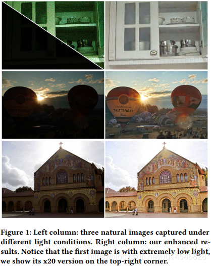
Figure 1 provides three natural images captured under challenging light conditions.

Concretely, the first case is with extremely low light. Severe noise and color distortion are hidden in the dark. By simply amplifying the intensity of the image, the degradations show up as given on the top-right corner.

The second image is photographed at sunset (weak ambient light), most objects in which suffer from backlighting. Imaging at noon facing to the light source (the sun) also hardly gets rid of the issue like the second case exhibits, although the ambient light is stronger and the scene is more visible. Note that those relatively bright regions of the last two photos will be saturated by direct amplification.

问题描述：

弱光情况下拍照可以采用直接增加亮度的（软件件）技术，但同样会引入新的问题：

1. 通过简单地放大图像的强度，会出现退化（噪声和颜色失真），就像右上角给出的那样；

2. 对于背光图像，放大图像的强度，会导致相对明亮的区域变得过曝光。

通过前两段，作者告诉我们，弱光图像增强问题是一件非常难的事情，值得研究。

Deep learning-based methods have revealed their superior performance in numerical low-level vision tasks, such as denoising and super-resolution, most of which need the training data with ground truth. For the target problem, say low-light image enhancement, no ground-truth real data exists, although the order of light intensity can be determined. Because, from the viewpoint of users, the favorite light levels for different people/requirements could be much diverse. In other words, one cannot say what light condition is the best/ground-truth. Therefore, it is not so felicitous to map an image only to a version with a specific level of light.

问题描述：基于深度学习方法的问题

基于深度学习的方法在去噪、超分辨等需要真实训练数据的低阶视觉任务中表现出了优越的性能。对于目标问题，比如弱光图像增强，虽然可以确定光强等级，但不存在真实数据。因为，从用户的角度来看，不同的人/需求最喜欢的光线水平可能是多种多样的。换句话说，谁也说不出什么光照条件是最好的，或者说 ground-truth 的确定因人而异。因此，仅将一幅图像映射到具有特定亮度的方法就不那么恰当了。

Based on the above analysis, we summarize challenges in lowlight image enhancement as follows:

• How to effectively estimate the illumination component from a single image, and flexibly adjust light levels?

• How to remove the degradations like noise and color distortion previously hidden in the darkness after lightening up dark regions?

• How to train a model without well-defined ground-truth light conditions for low-light image enhancement by only looking at two/several different examples?

In this paper, we propose a deep neural network to take the above concerns into account simultaneously

对上面问题描述的总结：

• 如何从一幅图像中有效地估计光照分量，灵活地调整光亮等级；

• 如何去除之前隐藏在黑暗区域的噪点、颜色失真等退化问题?

• 如何训练一个模型，在没有明确的 ground-truth 光照条件下，仅看两个/几个不同的例子，实现弱光图像增强?

解决这些问题，便是本文的 motivation。

算法回顾（Previous Arts ）

略

Methodology

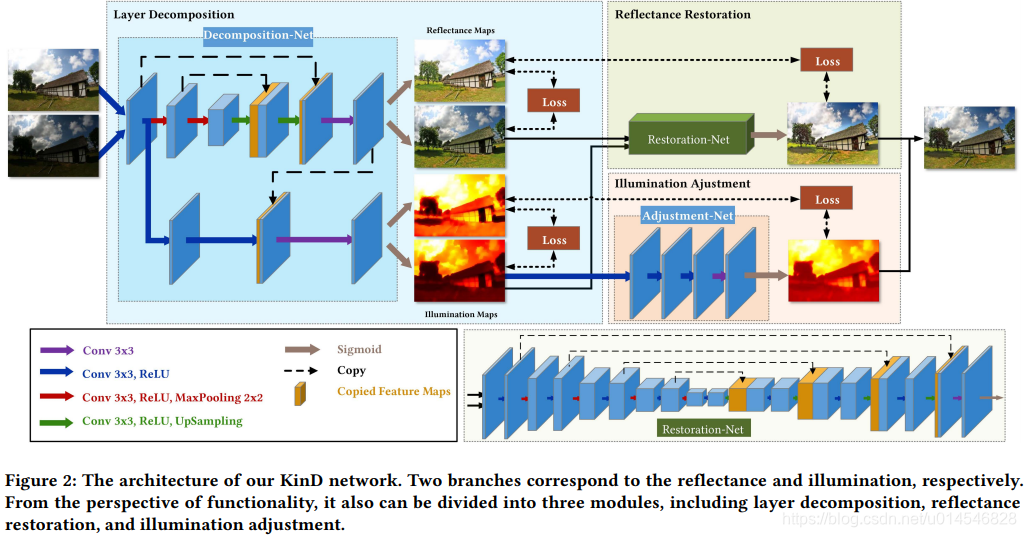
A desired low-light image enhancer should be capable to effectively remove the degradations hidden in the darkness, and flexibly adjust light/exposure conditions. We build a deep network, denoted as KinD, to achieve the goal. As schematically illustrated in Figure 2, the network is composed of two branches for handling the reflectance and illumination components, respectively. From the perspective of functionality, it also can be divided into three modules, including layer decomposition, reflectance restoration, and illumination adjustment. In the next subsections, we shall explain the details about the network.

一个理想的弱光图像增强算法应该能够有效地去除隐藏在黑暗中的退化，并灵活地调整光/曝光条件。

网络整体结构：

网络由两个支路组成，分别处理反射率和光照分量。

从功能上看，也可以分为三个模块，分别是图层分解、反射率恢复和光照调整。

Consideration & Motivation

Layer Decomposition.

The main drawback of plain methods comes from the blindness of illumination. Thus, it is key to obtain the illumination information. If having the illumination well-extracted from the input, the rest hosts the details and possible degradations, where the restoration (or degradation removal) can be executed on. In Retinex theory, an image $I$ can be viewed as a composition of two components, i.e. reflectance $R$ and illumination $L$ , in the fashion of $I = R \circ L$ , where $\circ$ designates the element-wise product. Further, decomposing images in the Retinex manner consequently decouples the space of mapping a degraded low-light image to a desired one into two smaller subspaces, expecting to be better and easier regularized/learned. Moreover, the illumination map is core to flexibly adjusting light/exposure conditions. Based on the above, the Retinex-based layer decomposition is suitable and necessary for the target task.

本文认为，如果从输入中很好地提取了光照，那么其余部分则承载了细节和可能的退化，在这里可以执行图像恢复 (或退化去除)。

在 Retinex 理论中，一幅图像可以被看作是由两部分组成的，即反射率 $R$ 和光照 $L$ ，按照的 $I = R \circ L$ 方式，这里 $\circ$ 是元素相乘。被 Retinex 理论分解的图像，解耦空间映射一个退化的弱光图像到一个期望的到两个理想的更小的子空间，从而使得正则化或学习更好更容易。

被分解的光照图像 illumination map 也是灵活调节亮度或曝光条件的核心部分。

这就是弱光图像增强为什么要两步走的原因。且基于 Retinex 的层分解对于目标任务是合适且必要的。

Data Usage & Priors.

There is no well-defined ground-truth for light conditions. Furthermore, no/few ground-truth reflectance and illumination maps for real images are available. The layer decomposition problem is in nature under-determined, thus additional priors/regularizers matter.

Suppose that the images are degradation-free, different shots of a certain scene should share the same reflectance. While the illumination maps, though could be intensively varied, are of simple and mutually consistent structure. In real situations, the degradations embodied in low-light images are often worse than those in brighter ones, which will be diverted into the reflectance component.

This inspires us that the reflectance from the image in bright light can perform as the reference (ground-truth) for that from the degraded low-light one to learn restorers.

One may ask that why not use synthetic data? Because it is hard to synthesize. The degradations are not in a simple form, and change with respect to different sensors. Please notice that the usage of reflectance (welldefined) totally differs from using images in (relatively) bright light as the reference of low light ones.

介绍了数据集的问题。

Illumination Guided Reflectance Restoration.

In the decomposed reflectance, the pollution of regions corresponding to darker illumination is heavier than that to brighter one. Mathematically, a degraded low-light image can be naturally modeled as $I=R\circ L+E$ , where $E$ designates the pollution component. By taking simple algebra steps, we have:

$I=R\circ L+E=\widetilde{R}\circ L=(R+\widetilde{E})\circ L=R\circ L + \widetilde{E}\circ L,$

where $\widetilde{R}$ stands for the polluted reflectance, and $\widetilde{E}$ is the degradation having the illumination decoupled. The relationship $E = \widetilde{E} \circ L$ holds. Taking the additive white Gaussian noise $E \sim \mathcal{N} (0, \sigma^2 )$ for an example, the distribution of $\widetilde{E}$ becomes much more complex and strongly relates to $L$ , i.e. $\sigma^2/L_i$ for each position $i$ . This is to say, the reflectance restoration cannot be uniformly processed over an entire image, and the illumination map can be a good guider.

One may wonder what if directly removing $E$ from the input $I$ ? For one thing, the unbalance issue still remains. By viewing from another point, the intrinsic details will be unequally confounded with the noise. For another thing, different from the reflectance, we no longer have proper references for degradation removal in this manner, since $L$ varies. Analogous analysis serves other types of degradation, like color-distortion.

本段给出了分解的数学表达式。并指出，反射率 reflectance 的恢复不能在整个图像上进行均匀处理，而光照图 illumination 可以作为一个很好的向导（）。

那为什么不直接从弱光图像 $I$ 中直接去除噪声 $E$ 呢？一方面，失衡问题仍然存在，图像中内在的细节与噪音混淆在一起。另一方面，去噪没有合适的参考图像。

Arbitrary Illumination Manipulation.

The favorite illumination strengths of different persons/applications may be pretty diverse. Therefore, a practical system needs to provide an interface for arbitrary illumination manipulation. In the literature, three main ways for enhancing light conditions are fusion, light level appointment, and gamma correction. The fusion-based methods, due to the fixed fusion mode, lack in the functionality of light adjustment. If adopting the second option, the training dataset has to contain images with target levels, limiting its flexibility. For gamma correction, although it can achieve the goal by setting different γ values, it may be unable to reflect the relationship between different light (exposure) levels. This paper advocates to learn a flexible mapping function from real data, which accepts users to appoint arbitrary levels of light/exposure.

不同的人/应用程序最喜欢的照明强度可能是非常不同的。因此，一个实际的系统需要提供一个任意照明操作的接口。在文献中，增强光条件的三种主要方法是融合、光级预约和伽马校正。基于融合的方法由于融合模式固定，缺乏光调节功能。如果采用第二种方法，训练数据集必须包含目标级别的图像，这限制了它的灵活性。对于伽马校正，虽然可以通过设置不同的静置值来达到目的，但可能无法反映不同光(曝光度)水平之间的关系。本文提倡从真实数据中学习一个灵活的映射函数，允许用户指定任意的光/曝光级别。

KinD Network

Inspired by the consideration and motivation, we build a deep neural network, denoted as KinD, for kindling the darkness. Below, we describe the three subnets in details from the functional perspective.

从三个网络结构展开介绍：图层分解网络、反射率恢复网络和亮度调节网络。

Layer Decomposition Net.

本段分为两部分，先介绍了损失函数的定义；然后介绍了网络结构。

损失函数：

Recovering two components from one image is a highly ill-posed problem. Having no ground-truth information guided, a loss with well-designed constraints is important. Fortunately, we have paired images with different light/exposure configurations $[I_l , I_h]$ . Recall that the reflectance of a certain scene should be shared across different images, we regularize the decomposed reflectance pair $[R_l , R_h]$ to be close (ideally the same if degradation-free). Furthermore, the illumination maps $[L_l , L_h]$ should be piece-wise smooth and mutually consistent.

The following terms are adopted. We simply use $\mathcal{L}^{LD}_{rs} := \left\| R_l-R_h \right \|_1$ to regularize the reflectance similarity, where $\left \| \cdot \right \|$ means the $\ell^1$ norm.

The illumination smoothness is constrained by $\mathcal{L}^{LD}_{is} := \left\| \dfrac{\nabla L_l}{max(|\nabla I_l, \epsilon )} \right \|_1 + \left\| \dfrac{\nabla L_h}{max(|\nabla I_h, \epsilon )} \right \|_1$ , where $\nabla$ stands for the first order derivative operator containing $\nabla x$ (horizontal) and $\nabla y$ (vertical) directions. In addition, $\epsilon$ is a small positive constant (0.01 in this work) for avoiding zero denominator, and $|\cdot |$ means the absolute value operator. This smoothness term measures the relative structure of the illumination with respect to the input. 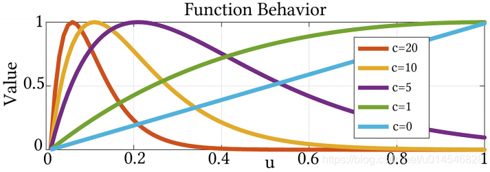For a location on an edge in $I$ , the penalty on $L$ is small; while for a location in a flat region in $I$ , the penalty turns to be large.

As for the mutual consistency, we employ $\mathcal{L}^{LD}_{mc}:= \| \mathcal{M}\circ \exp(-c\cdot \mathcal{M})\|_1$ with $\mathcal{M} := |\nabla L_l | + |\nabla L_h |$ . Figure 4 depicts the function behavior of $u \cdot \exp(-c \cdot u)$ , where $c$ is the parameter controlling the shape of function. As can be seen from Figure 4, the penalty first goes up but then drops towards 0 as $u$ increases. This characteristic well fits the mutual consistency, i.e. strong mutual edges should be preserved while weak ones depressed. We notice that setting $c = 0$ leads to a simple $\ell^1$ loss on $\mathcal{M}$ .

Besides, the decomposed two layers should reproduce the input, which is constrained by the reconstruction error, say $\mathcal{L}^{LD}_{ec} := \| I_l-R_l \circ L_l \|_1 + \| I_h-R_h \circ L_h \|_1$ .

As a result, the loss function of layer decomposition net is as follows:

$\mathcal{L}^{LD}:=\mathcal{L}^{LD}_{rec}+0.01\mathcal{L}^{LD}_{rs}+0.15\mathcal{L}^{LD}_{is}+0.2\mathcal{L}^{LD}_{mc}.$

Figure 4: The behavior of function $v=u \cdot \exp(-c \cdot u)$ . The parameter $c$ controls the shape of function.

包括四个部分（损失函数的定义，是根据一些先验知识给出的）：

1. reflectance similarity ：前面已经分析过了，对于强光图像和弱光图像，二者的反射率是近似相同的（二者只是光照不同罢了），因此损失函数定义为 $\mathcal{L}^{LD}_{rs} := \left\| R_l-R_h \right \|_1$ ；

2. illumination smoothness ：前面分析过，光照图像可以用输入图像进行引导，在输入图像强边缘区，光照发生较大变化；在弱边缘区，光照可以认为也是平滑的，因此损失函数定义为 $\mathcal{L}^{LD}_{is} := \left\| \dfrac{\nabla L_l}{max(|\nabla I_l, \epsilon )} \right \|_1 + \left\| \dfrac{\nabla L_h}{max(|\nabla I_h, \epsilon )} \right \|_1$ 。注意到，当 $\nabla I$ 较大时（边缘），使得损失函数值很小，此时对 $\nabla L$ 的约束较轻；当 $\nabla I$ 较小时（平滑），使得损失函数值增大，此时要求 $\nabla L$ 必须很小，才能减小损失函数值。这样，光照图像 $L$ 就和输入图像 $I$ 有一个相关的结构。

3. mutual consistency ：这个损失函数是说， $[L_l , L_h]$ 二者的结构应该是一致的。那为什么要定义成 $\mathcal{L}^{LD}_{mc}:= \| \mathcal{M}\circ \exp(-c\cdot \mathcal{M})\|_1$ 这个样子呢？图 4 给出的是一个一维的例子。发现，当 $u$ 近似为 0 或者比较大时，这个损失函数的值比较小，对应到二维情况就是 $\mathcal{M} := |\nabla L_l | + |\nabla L_h |$ 近似 0 或者较大时（ $[L_l , L_h]$ 二者的梯度都很小或者都很大时），约束较小；而当 $u$ 在 0 和较大之间时，这个损失函数的值比较大，对应到二维情况就是 $\mathcal{M} := |\nabla L_l | + |\nabla L_h |$ 在 0 和较大之间时（ $[L_l , L_h]$ 二者的梯度一个比较小，一个比较大），此时约束就很大，迫使 $[L_l , L_h]$ 其中一个和另一个相近。

4. reconstruction error ：即生成的 $[R_l , R_h]$ 和 $[L_l , L_h]$ 反过来合成的两个新图，应分别于 $[I_l , I_h]$ 相似，即 $\mathcal{L}^{LD}_{ec} := \| I_l-R_l \circ L_l \|_1 + \| I_h-R_h \circ L_h \|_1$ 。

最后，图层分解网络的损失函数就是 4 者相加。

下面是图层分解网络结构：

The layer decomposition network contains two branches corresponding to the reflectance and illumination, respectively. The reflectance branch adopts a typical 5-layer U-Net [25], followed by a convolutional (conv) layer and a Sigmoid layer. While the illumination branch is composed of two conv+ReLU layers and a conv layer on concatenated feature maps from the reflectance branch (for possibly excluding textures from the illumination), finally followed by a Sigmoid layer.

图层分解网络分为两个路径：

1. reflectance branch ：5-layer U-Net + a conv layer + Sigmoid ；

2. illumination branch ：two （conv+ReLU layers） + a conv layer（级联从 reflectance branch 来的特征图，目的是为了从光照中排除纹理）+ Sigmoid。

Reflectance Restoration Net.

The reflectance maps from lowlight images, as shown in Figures 3 and 5, are more interfered by degradations than those from bright-light ones. Employing the clearer reflectance to act as the reference (informal ground-truth) for the messy one is our principle.

For seeking a restoration function, the objective turns to be simple as follows:

$\mathcal{L}^{RR}:=\|\hat{R}-R_h\|^2_2-SSIM(\hat{R},R_h)+\|\nabla \hat{R}-\nabla R_h\|^2_2,$

where $SSIM(\cdot, \cdot)$ is the structural similarity measurement, $\hat{R}$ corresponds to the restored reflectance, and $\| \cdot \|_2$ means the $\ell^2$ norm (MSE). The third term concentrates on the closeness in terms of textures.

This subnet is similar to the reflectance branch in the layer decomposition subnet, but deeper. The schematic configuration is given in Figure 2.

We recall that the degradation distributes in the reflectance complexly, which strongly depends on the illumination distribution. Thus, we bring the illumination information into the restoration net together with the degraded reflectance.

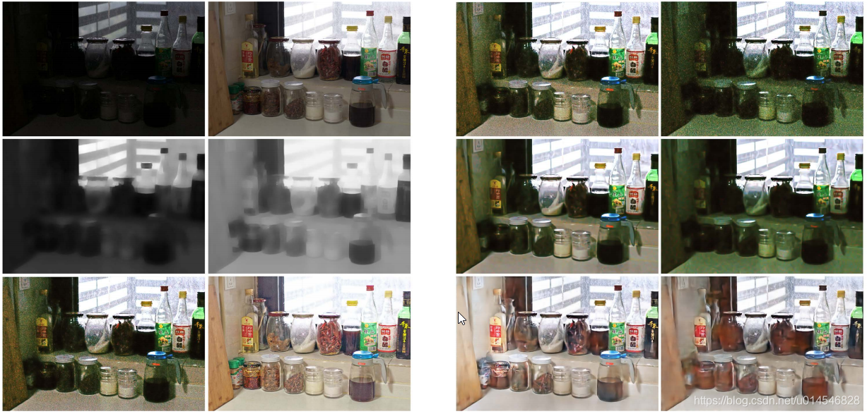
The effectiveness of this operation can be observed in Figure 5. In the two reflectance maps with different degradation (light) levels, the results by BM3D can fairly remove noise (without regarding the color distortion in nature). The blur effect exists almost everywhere. In our results, the textures (the dust/water-based stains for example) of the window region, which is originally bright and barely polluted, keeps clear and sharp, while the degradations in the dark region get largely removed with details (e.g. the characters on the bottles) very well maintained. Besides, the color distortion is also cured by our method.

（ $\leftarrow$ ）Figure 3: Left column: Lower light input and its decomposed illumination and (degraded) reflectance maps. Right column: Brighter input and its corresponding maps. Three rows respectively correspond to inputs, illumination maps, and reflectance maps. These are testing images.

（ $\rightarrow$ ）Figure 5: The polluted reflectance maps (top), and their results by BM3D (middle) and our reflectance restoration net (bottom). The right column corresponds to a heavier degradation (a lower light) level than the left. These are testing images.

反射率恢复网络：整个一大段，看起来比较费劲，我这里把它分解为 5 部分内容

1. 网络的原则是：采用较清晰的反射率作为较杂乱的反射率的参考。

2. 损失函数： $\mathcal{L}^{RR}:=\|\hat{R}-R_h\|^2_2-SSIM(\hat{R},R_h)+\|\nabla \hat{R}-\nabla R_h\|^2_2,$

3. 网络结构：U-Net （更多层）。

4. 需要注意的是，文章解释了为什么反射率恢复网络还有引入亮度图像 $[L_l , L_h]$ （从图2可以看到这个连接）。这是因为，前面说过，噪声和颜色失真最主要出现在弱光照的区域，即衰减的分布依赖于照明分布。因此，将光照信息与反射系数降低一起带入恢复网中。

5. 最后，用图 5 进行了效果说明。传统的 BM3D 会使图像出现模糊现象。而本文的方法，保持图像的清晰和锐化。

Illumination Adjustment Net.

There does not exist a ground-truth light level for images. Therefore, for fulfilling diverse requirements, we need a mechanism to flexibly convert one light condition to another. We have paired illumination maps. Even though without knowing the exact relationship between the paired illuminations, we can roughly calculate their ratio of strength, i.e. $\alpha$ by $mean(L_t /L_s )$ where the division is element-wise. This ratio can be used as an indicator to train an adjustment function from a source light $L_s$ to a target one $L_t$ . If adjusting a lower level of light to a higher one, $\alpha > 1$ , otherwise $\alpha \leq 1$ . In the testing phase, $\alpha$ can be specified by users.

The network is lightweight, containing 3 conv layers (two conv+ReLu, and one conv) and 1 Sigmoid layer. We notice that the indicator $\alpha$ is expanded to a feature map, acting as a part of input for the net.

The following is the loss for illumination adjustment net:

$\mathcal{L}^{IA}:=\|\hat{L}-L_t\|^2_2 + \| |\nabla \hat{L}_t|-|\nabla L_t| \|^2_2,$

where $L_t$ can be $L_h$ or $L_l$ , and $\hat{L}$ is the adjusted illumination map from the source light ( $L_h$ or $L_l$ ) towards the target one.

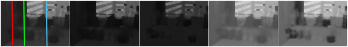
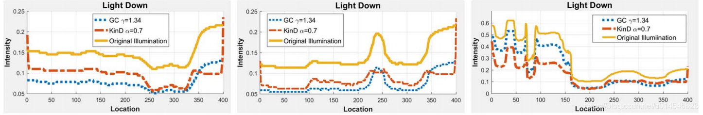
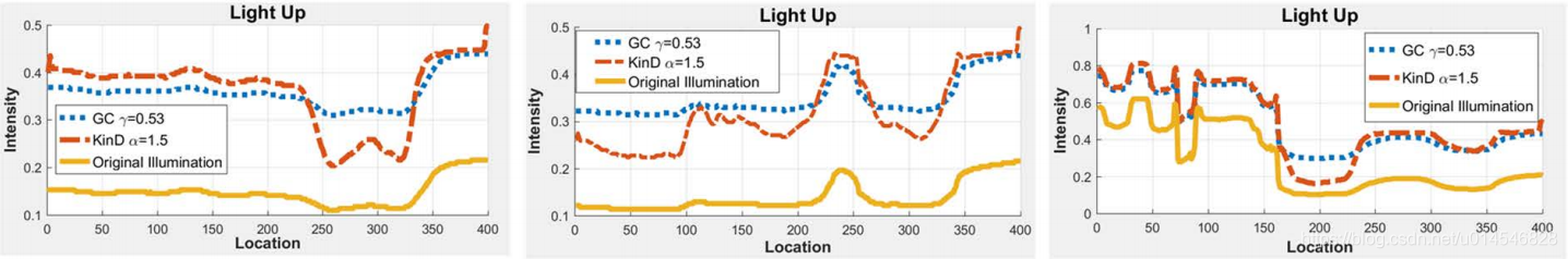
Figure 6 shows the difference between our learned adjustment function and gamma correction. For comparison fairness, we tune the parameter $\gamma$ for gamma correction to reach a similar overall light strength with ours via $\gamma = \| log(\hat{L}) \|_1/\| log(L_s ) \|_1$ . We consider two adjustments without loss of generality, including one light down and one light up. Figure 6 (a) depicts the source illumination, (b) and (d) are the adjusted results by gamma correction, while (c) and (e) are ours. To more clearly show the difference, we plot the 1D intensity curves at $x = 100, 200, 400$ . As for the light-down case, our learned manner decreases more than gamma correction in intensity on relatively bright regions, while less or about the same on dark regions. Regarding the light-up case, the opposite trend appears. In other words, our method increases less the light on relatively dark regions, while more or about the same on bright regions. The learned manner is more corroborative with actual situations.

Furthermore, the $\alpha$ fashion is more convenient than the $\gamma$ way for users to manipulate. For instance, setting $\alpha$ to 2 means turns the light 2X up.

（a）Original illu. （b） $\gamma$ correction （c） Ours （d） $\gamma$ correction （e） Ours

（f）Light-Down, x=100 （g）Light-Down, x=200 （h）Light-Down, x=400

（i）Light-Up, x=100 （j）Light-Up, x=200 （k）Light-Up, x=400

亮度调剂网络：也是一整段，我把它分解为 5 部分：

1. 参数 $\alpha$ ：由于给定的两个图像是相对强弱的。那么，输出的图像，是以强光图像为目标呢，还是以弱光图像为目标呢？如果用户是想将弱光图像强化，就设置强光图像为目标，反之，以弱光图像为目标。这个操作可以根据用户需求而自己设置。怎么设置呢？就是通过参数 $\alpha =mean(L_t /L_s )$ 来实现。其中， $L_t$ 表示目标图像； $L_s$ 表示原图像（例如，若对弱光图像强化，则 $L_t=L_h, ~L_s=L_l$ ）。

2. 亮度调剂网络结构： two （conv+ReLu ）+ one conv + Sigmoid 。注意到 $\alpha$ 被扩展为一个特征图，作为网络输入的一部分。

3. 亮度调剂损失函数： $\mathcal{L}^{IA}:=\|\hat{L}-L_t\|^2_2 + \| |\nabla \hat{L}_t|-|\nabla L_t| \|^2_2,$ 即输出图像 $\hat{L}$ 应和目标图像相似，且边缘也相似。

4. 与 $\gamma$ 变换的对比：图 6 是本文亮度调节方法与 $\gamma$ 变换结果的对比。对比实验包括亮度降低（以弱光图像为目标）和亮度提升（以强光图像为目标）两个方面。为了更清晰说明情况，(f)-(k) 的曲线图给出了各个图像中 $x = 100, 200, 400$ 这三列像素的曲线对比。

从 (f)-(h) 可以看出，对于亮度降低情况中，在相对明亮的区域，KinD 学习的方式在强度上比 $\gamma$ 变换减少更多，而在黑暗的区域减少较小或与 $\gamma$ 变换差不多相同。

从 (i)-(k) 可以看出，对于亮度提升情况中，KinD 方法在相对暗的区域对光的增强小于 $\gamma$ 变换，而在明亮的区域的光强调整比 $\gamma$ 变换增加更多或差不多相同。

总之，KinD 的方法在亮度调节上，比 $\gamma$ 变换得到的亮度对比度更高。

5. 作者最后指出，亮度调节可以通过调节 $\alpha$ 实现。 $\alpha$ 是参与网络训练的， $\alpha$ 被扩展为一个特征图，作为网络输入的一部分。例如，当 $L_t=L_h, ~L_s=L_l$ ，设置 $\alpha =2$ ，表示图像的亮度增加 2 倍。

Experimental Validation

Implementation Details

We use the LOL dataset as the training dataset, which includes 500 low/normal-light image pairs. In the training, we merely employ 450 image pairs, and no synthetic images are used.

For the layer decomposition net, batch size is set to be 10 and patch-size to be 48x48.

While for the reflectance restoration net and illumination adjustment net, batch size is set to be 4 and patch-size to be 384x384.

We use the stochastic gradient descent (SGD) technique for optimization. The entire network is trained on a Nvidia GTX 2080Ti GPU and Intel Core i7-8700 3.20GHz CPU using the Tensorflow framework.

Performance Evaluation

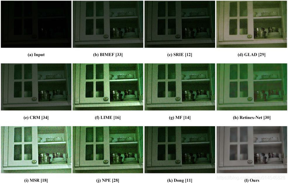
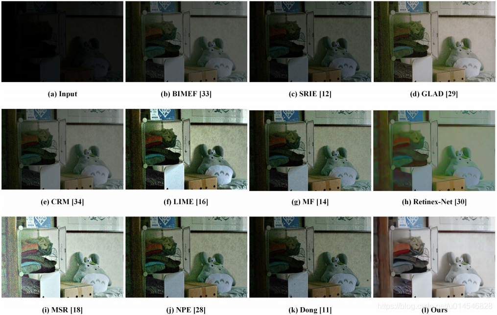
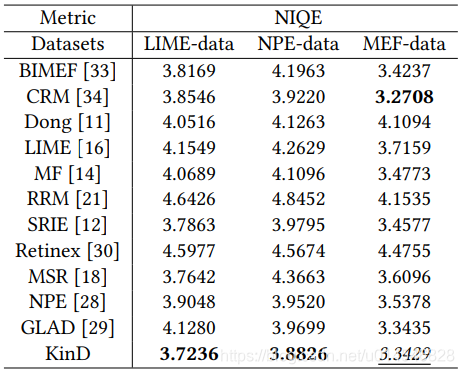
We evaluate our method on widely-adopted datasets, including LOL [30], LIME [16], NPE [28], and MEF [7]. Four metrics are adopted for quantitative comparison, which are PSNR, SSIM, LOE [28], and NIQE [23]. A higher value in terms of PSNR and SSIM indicates better quality, while, in LOE and NIQE, the lower the better. The state-of-the-art methods of BIMEF [33], SRIE [12], CRM [34], Dong [11], LIME [16], MF [14], RRM [21], Retinex-Net [30], GLAD [29], MSR [18] and NPE [28] are involved as the competitors.

Figure 7: Visual comparison with state-of-the-art low-light image enhancement methods.

Figure 8: Visual comparison with state-of-the-art low-light image enhancement methods.

Table 2: Quantitative comparison on LIME, NPE, and MEF datasets in terms of NIQE. The best results are highlighted in bold.

数据集：

LOL [30] : Deep Retinex Decomposition for Low-Light Enhancement. 2018 British Machine Vision Conference.

LIME [16] : LIME: Low-light Image Enhancement via Illumination Map Estimation. IEEE TIP (2017).

NPE [28] : Naturalness preserved enhancement algorithm for non-uniform illumination images. IEEE TIP (2013).

MEF [7] : Powerconstrained contrast enhancement for emissive displays based on histogram equalization. IEEE TIP (2012).

评价方法：

LOE [28] : Naturalness preserved enhancement algorithm for non-uniform illumination images. IEEE TIP (2013).

NIQE [23] : Making a completely blind image quality analyzer. IEEE Signal Processing Letters (2013).

对比方法：

BIMEF [33] : A Bio-Inspired Multi-Exposure Fusion Framework for Low-light Image Enhancement. arXiv (2017). (code)

SRIE [12] ：A Weighted Variational Model for Simultaneous Reflectance and Illumination Estimation. 2016 CVPR. (code)

CRM [34] : A New Low-Light Image Enhancement Algorithm Using Camera Response Model. 2018 ICCVW. (code)

Dong [11] : Fast efficient algorithm for enhancement of low lighting video. 2011 ICME. (code)

LIME [16] : LIME: Low-light Image Enhancement via Illumination Map Estimation. IEEE TIP (2017). (code)

MF [14] : A fusion-based enhancing method for weakly illuminated images. Signal Processing (2016). (code)

RRM [21] : Structure-Revealing Low-Light Image Enhancement Via Robust Retinex Model. IEEE TIP (2018). (code)

Retinex-Net [30] : Deep Retinex Decomposition for Low-Light Enhancement. 2018 British Machine Vision Conference. (code)

GLAD [29] : GLADNet: Low-Light Enhancement Network with Global Awareness. 2018 In IEEE International Conference on Automatic Face & Gesture Recognition. (code)

MSR [18] : A multiscale retinex for bridging the gap between color images and the human observation of scenes. IEEE TIP (2012). (code)

NPE [28] : Naturalness preserved enhancement algorithm for non-uniform illumination images. IEEE TIP (2013). (code)

——————————————————————————

补充方法：

DeepUPE : Underexposed photo enhancement using deep illumination estimatio. 2019 CVPR. (code)

Zero-reference deep curve estimation for low-light image enhancement. 2020 arxiv. (code) (project)

——————————————————————————

KinD++

网络结构对比

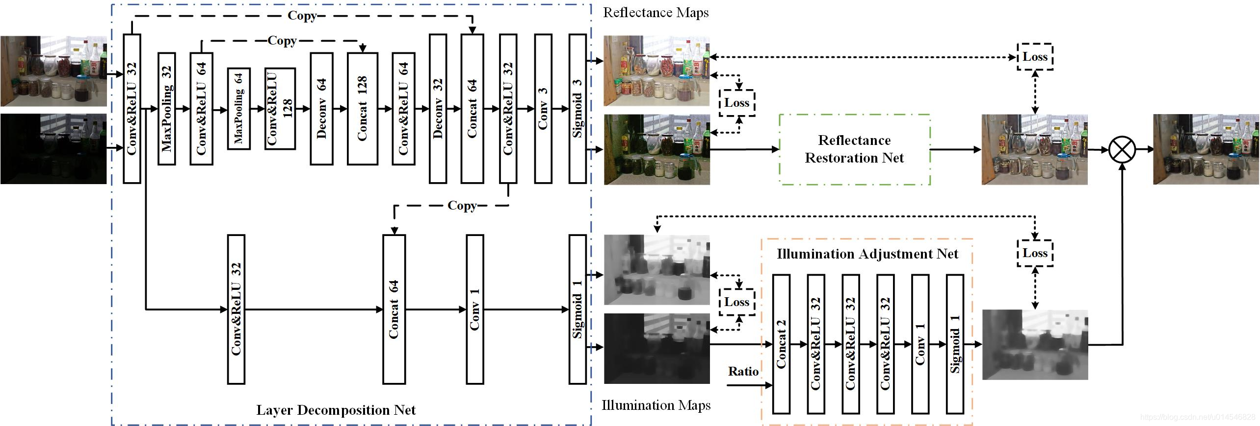
从整体上看，跟 KinD 基本相同。注意 ratio $\alpha$ 在这个图中画出来了（前面图 2 作者忘记画这个输入了）。

KinD++ 与 KinD 不同的地方，表现在反射率恢复网络，如下图。

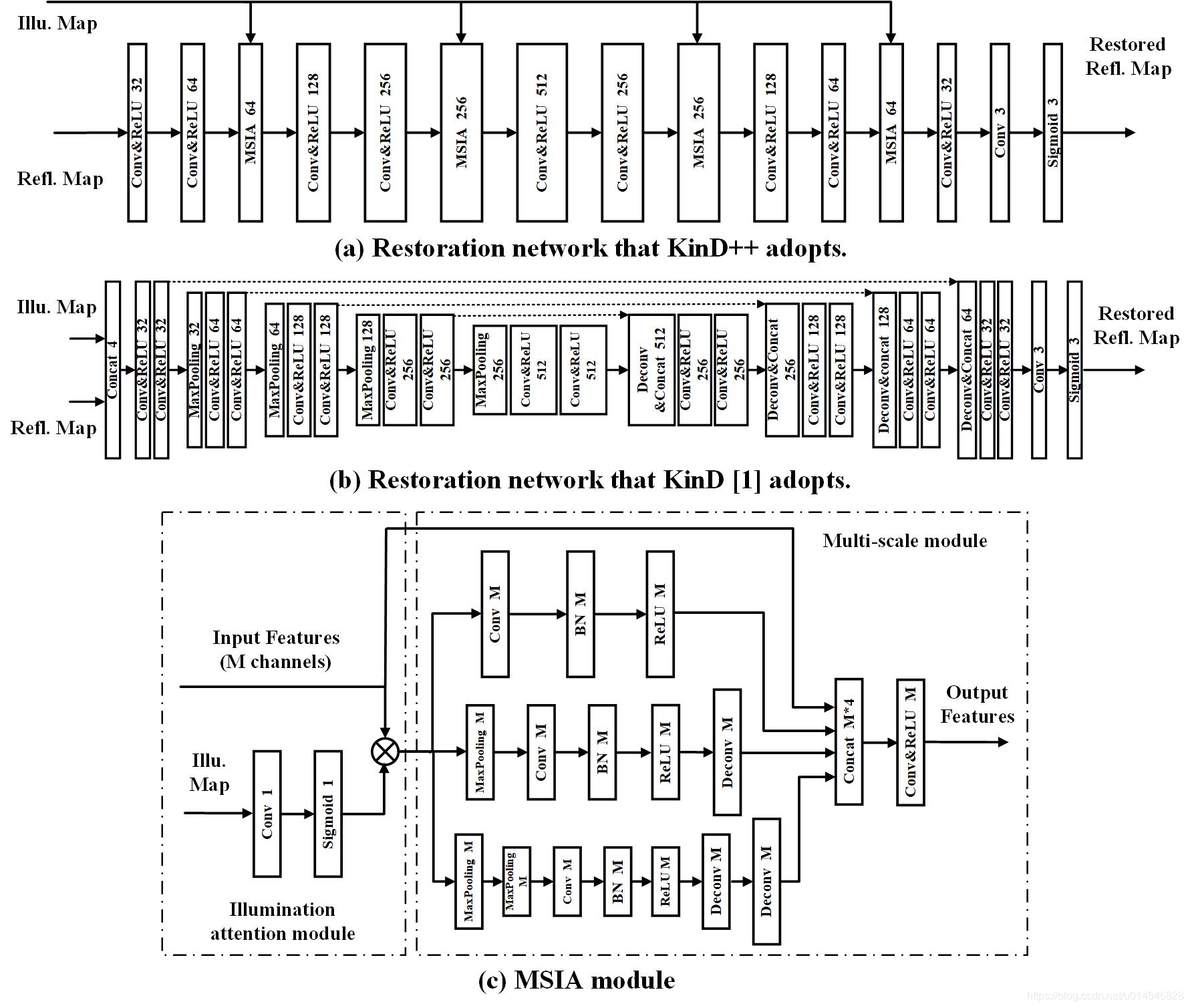
上图（a）和（b）是 KinD++ 与 KinD 之间的对比。

在 KinD++ 中，反射率恢复网络没有采用 U-Net，整个网络过程图像的空间分辨率保持不变，并引入了多尺度亮度注意力（MSIA）模块，如图（c）所示。

NIQE code

Non-reference metric NIQE is adopted for quantitative comparison. The original code for computing NIQE is here. To improve the robustness, we follow the author's code and retrain the model parameters by extending 100 high-resolution natural images from PIRM dataset. Put the original 125 images and additional 100 images (dir: PIRM_dataset\Validation\Original) into one folder 'data', then run

[mu_prisparam cov_prisparam]  = estimatemodelparam('data',96,96,0,0,0.75);

After retrained, the file 'modelparameters_new.mat' will be generated. We use this model to evaluate all results.

Phoenixtree_DongZhao

关注

4
点赞
踩
31

收藏

觉得还不错? 一键收藏
0
评论
MyDLNote-Enhancement: Kindling the Darkness: a Practical Low-light Image Enhancer （后附 KinD ++）

Kindling the Darkness: a Practical Low-light Image Enhancer[paper] :https://arxiv.org/pdf/1905.04161v1.pdf[Tensorflow] :https://github.com/zhangyhuaee/KinDAbstractImages captured under low-light conditions often suffer from (partially) p...
复制链接

扫一扫