


1.%为注释
>> 1 == 2 % false
ans = 0
2.~= 为不等于号
>> 1~=2
ans = 1
3.&&逻辑与
>> 1&&0
ans = 0
4.||或运算
>> 1||0
ans = 1
5.抑或运算
>> xor(1,0)
ans = 1
6.分号关闭提示

7.提取变量的值
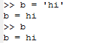
8.disp显示变量
>> a =pi
a =  3.1416
>> disp(sprintf('6 decimals: %0.6f',a))
6 decimals: 3.141593
9.改变输出格式 为长款数字 还是 短款数字
>> format long
>> a
a =  3.141592653589793
>> format short
>> a
a =  3.1416
10.定义矩阵
>> A = [1,2;3,4;5,6]
A =

   1   2
   3   4
   5   6
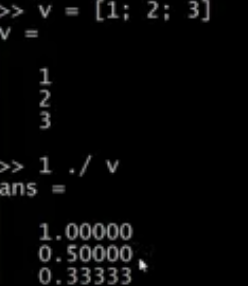
11.定义向量
>> v=[1 ;2 ;3]
v =
   1
   2
   3
12.从1开始每次增加0.1,增加到2
>> v= 1:0.1:2
v =
    1.0000    1.1000    1.2000    1.3000    1.4000    1.5000    1.6000    1.7000    1.8000    1.9000    2.0000
13.构建数值都为1的矩阵
>> ones(2,3)
ans =

   1   1   1
   1   1   1

>> 2*ones(2,3)
ans =

   2   2   2
   2   2   2
14.构建数值都为0的矩阵
>> zeros(1,3)
ans =

   0   0   0
15.构建数值随机的矩阵
0到1数值随机
>> rand(3,3)
ans =

   0.913102   0.320718   0.995509
   0.038083   0.707257   0.169677
   0.444543   0.864916   0.689890
符合高斯分布的随机数值(平均值为0,方差和标准差为1)
>> randn (1,3)
ans =

  -0.71084   0.65244  -0.30712
16.画图
首先计算大量随机数值 w = -6 +sqrt(10)*(randn(1,10000))
>> hist(w) 画出随机值对应的数量直方图

hist(w,30) 30个区间
将区间分的更精细

17.构建单位矩阵
>> eye(4)
ans =

Diagonal Matrix

   1   0   0   0
   0   1   0   0
   0   0   1   0
   0   0   0   1
18.帮助命令

19.矩阵大小计算
>> A =[1 2;3 4;5 6]
A =

   1   2
   3   4
   5   6
返回的A的大小 为1行2列的矩阵
>> size(A)
ans =

   3   2
返回第一个行数
>> size(A,1)
ans =  3
返回第二个列数
>> size(A,2)
ans =  2
20.计算向量长度
>> v=[1 2 3 4]
v =

   1   2   3   4

>> length(v)
ans =  4
21.数据加载
>> cd 'E:\Coursera_ml_exr\machine-learning-ex1\ex1'
显示文件夹内容
>> dir
.                       ex1.m                   featureNormalize.m      normalEqn.m
..                      ex1_multi.m             gradientDescent.m       plotData.m
computeCost.m           ex1data1.txt            gradientDescentMulti.m  submit.m
computeCostMulti.m      ex1data2.txt            lib                     warmUpExercise.m
加载数据
load q1y.dat % alternatively, load('q1y.dat')
显示当前可用变量
who % list variables in workspace
显示当前可用变量的详细细节
whos % list variables in workspace (detailed view)
删除对应变量
clear q1y % clear command without any args clears all vars
v取前十个变量
v = q1x(1:10); % first 10 elements of q1x (counts down the columns)
将变量保存
save hello.mat v; % save variable v into file hello.mat
将变量存为文本文件
save hello.txt v -ascii; % save as ascii
取出第3行第2列的数值
A(3,2) % indexing is (row,col)
取出第2行所有数值
A(2,:)  % get the 2nd row.
        % ":" means every element along that dimension
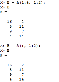
取出第2列所有数值
A(:,2) % get the 2nd col
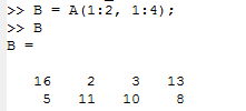
取出第一行 和 第三行 所有数值
A([1 3],:) % print all the elements of rows 1 and 3
将第二列 赋值为新的值
A(:,2) = [10; 11; 12] % change second column

增加新的一列
A = [A, [100; 101; 102]]; % append column vec

将所有数值 放入一个列向量中
A(:) % Select all elements as a column vector.

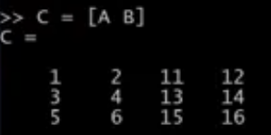
左右连接两个矩阵
C = [A B]  % concatenating A and B matrices side by side
C = [A, B] % concatenating A and B matrices side by side
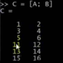
上下连接两个矩阵
C = [A; B] % Concatenating A and B top and bottom
22.矩阵操作
%% matrix operations
矩阵乘法
A * C % matrix multiplication
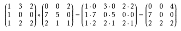
矩阵元素对应相乘(哈达马积(Hadamard product))
    A .* B % element-wise multiplication

% A .* C  or A * B gives error - wrong dimensions(需要相乘的两个矩阵 维度相同)
矩阵平方
A .^ 2 % element-wise square of each element in A
矩阵对应元素除法
1./v % element-wise reciprocal
矩阵对应元素log10
log(v) % functions like this operate element-wise on vecs or matrices
矩阵对应元素log自然对数
exp(v)
矩阵对应元素取绝对值
abs(v)
矩阵对应元素加副号
-v % -1*v
矩阵对应元素加一
(length返回多少个元素,也就是多少行。即三行一列)
v + ones(length(v), 1)
v+1也是一样的结果
% v + 1 % same

矩阵转置
A’ % matrix transpose
常用函数介绍
%% misc useful functions
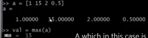
取最大或最小值
% max (or min)
取最大值
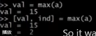
val = max(a)
返回最大值与最大值对应的角标
[val,ind] = max(a) % val - maximum element of the vector a and index - index value where maximum occur
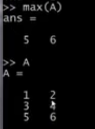
假如A是矩阵,返回每一列的最大值
val = max(A) % if A is matrix, returns max from each column
比较每一个值 是否小于3
% compare values in a matrix & find
a < 3 % checks which values in a are less than 3
比较每一个值 是否小于3,并返回对应值的角标
find(a < 3) % gives location of elements less than 3
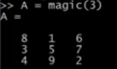
magic矩阵每一行相加 每一列,对角线相加 的总和相同
A = magic(3) % generates a magic matrix - not much used in ML algorithms
找到A中大于等于7的行标与列标
[r,c] = find(A>=7) % row, column indices for values matching comparison

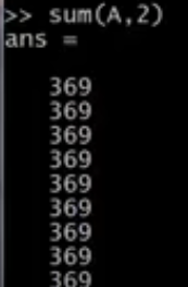
所有元素相加
% sum, prod
sum(a)
返回所有元素连乘乘积
prod(a)
向上取整or向下取整
floor(a) % or ceil(a)
3*3的随机矩阵对应元素相乘
max(rand(3),rand(3))
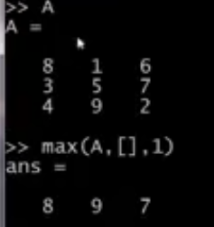
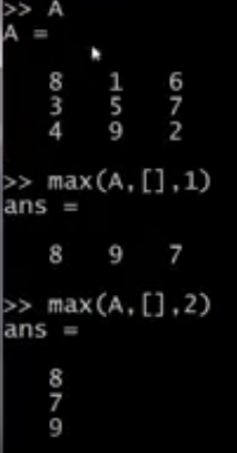
矩阵A每一列的最大值
max(A,[],1) - maximum along columns(defaults to columns - max(A,[]))
矩阵A每一行的最大值
max(A,[],2) - maximum along rows
整个矩阵中所有元素中的最大值
max(max(A))
or
max(A(:))
将A变成向量求解
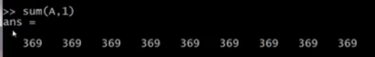
按行加和
A = magic(9)
sum(A,1)
按列加和
sum(A,2)
主对角线元素加和
sum(sum( A .* eye(9) ))

副对角线元素加和
sum(sum( A .* flipud(eye(9)) ))
求逆矩阵
% Matrix inverse (pseudo-inverse)
pinv(A) % inv(A’*A)*A’
画图
横轴为t向量 纵轴为y
%% plotting
t = [0:0.01:0.98];
y1 = sin(2*pi*4*t);
plot(t,y1);

让当前图片保持不动 再增加新的图像
y2 = cos(2*pi*4*t);
hold on;  % "hold off" to turn off
plot(t,y2,'r');
横轴标注
xlabel('time');
纵轴标注
ylabel('value');
图例
legend('sin','cos');
标题
title('my plot');

输出为png文件
print -dpng 'myPlot.png'
关闭图片窗口
close; % or, "close all" to close all figs
打开一号窗口figure(1) 二号窗口figure(2)
figure(1); plot(t, y1);
figure(2); plot(t, y2);
将图片变为1行2列的网格,第一个放一张图
>> subplot(1,2,1);  % Divide plot into 1x2 grid, access 1st element
>> plot(t,y1);
第二个放一张图
>> subplot(1,2,2);  % Divide plot into 1x2 grid, access 2nd element
>> plot(t,y2);

改变横轴 纵轴范围
axis([0.5 1 -1 1]); % change axis scale
清空画布
clf;
将矩阵变成图片
%% display a matrix (or image)
>> A
A =

   17   24    1    8   15
   23    5    7   14   16
    4    6   13   20   22
   10   12   19   21    3
   11   18   25    2    9
imagesc(magic(15)),

增加侧边栏,颜色调,并将颜色改为灰度
imagesc(A),colorbar, colormap gray;

同时运行多条命令且显示提示,使用“,”
% comma-chaining function calls.
a=1,b=2,c=3
a=1;b=2;c=3;
23.控制语句Control Statements: for, while, if statement
输出2的i次方
>> for i=1:10,
    v(i) = 2^i;
end;
>> v
v =

      2      4      8     16     32     64    128    256    512   1024
另一种循环1到10写法
>> indices = 1:10
indices =

    1    2    3    4    5    6    7    8    9   10

>> for i=indices,
disp(i);
end;
 1
 2
 3
 4
 5
 6
 7
 8
 9
 10
将前5个变成100的循环,使用while循环
>> i = 1;
>> while i <= 5,
  v(i) = 100;
  i = i+1;
end
>> v
v =

    100    100    100    100    100     64    128    256    512   1024
将前5个变成999的循环,使用break语句
i = 1;
while true,
  v(i) = 999;
  i = i+1;
  if i == 6,
    break;
  end;
end
>> v
v =

    999    999    999    999    999     64    128    256    512   1024
if判断语句
>> if v(1)==1,
  disp('The value is one!');
elseif v(1)==2,
  disp('The value is two!');
else
  disp('The value is not one or two!');
end
The value is not one or two!
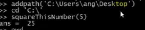
函数
function y = squareThisNumber(x)
y = x^2;
切换到对应路径,才能使用该函数
% Navigate to directory:
    cd /path/to/function

    % Call the function:
    functionName(args)
将路径加入octave,以后切换路径后,也能使用该函数
% To add the path for the current session of Octave:
addpath('/path/to/function/')
% To remember the path for future sessions of Octave, after executing addpath above, also do:
savepath
多返回值函数
function [y1, y2] = squareandCubeThisNo(x)
y1 = x^2
y2 = x^3
调用该函数
[a,b] = squareandCubeThisNo(x)
调用损失函数
损失函数文件

>> X = [1 1;1 2;1 3]
X =
   1   1
   1   2
   1   3

>> y = [1;2;3]
y =

   1
   2
   3

>> theta = [0;0]
theta =

   0
   0

>> j = computeCost(X, y, theta)
j =  2.3333
矩阵平方
A .^ 2 % element-wise square of each element in A
练习题:


octave编程示例:


提交作业


 2961
2961


 被折叠的 条评论
为什么被折叠?
被折叠的 条评论
为什么被折叠?
 到【灌水乐园】发言


