理解ggplot2颜色的标尺函数（scale_color_*,scale_color_*）

关于颜色的标尺函数在ggplot2中竟然多达22种，如此多的标尺函数未免使人感到疑惑

library(ggplot2)
grep('scale_color_*', x = ls('package:ggplot2'), value = TRUE)#在这里fill同理

[1] “scale_color_binned” “scale_color_brewer”
[3] “scale_color_continuous” “scale_color_date”
[5] “scale_color_datetime” “scale_color_discrete”
[7] “scale_color_distiller” “scale_color_fermenter”
[9] “scale_color_gradient” “scale_color_gradient2”
[11] “scale_color_gradientn” “scale_color_grey”
[13] “scale_color_hue” “scale_color_identity”
[15] “scale_color_manual” “scale_color_ordinal”
[17] “scale_color_steps” “scale_color_steps2”
[19] “scale_color_stepsn” “scale_color_viridis_b”
[21] “scale_color_viridis_c” “scale_color_viridis_d”

对颜色标尺函数的理解

让我们直入正题，虽然ggplot2拥有多达22种的标尺函数，但我们可以根据关键性质（一共分为三种），这样我们可以大体知道在不同的情形下具体使用哪个标尺函数。

1. 数据映射的自然属性：
   aes()图形映射里描述的数据是连续的还是离散的？连续的典型如时间，温度，长度，离散的典型如分类结果ABCD。
2. 颜色空间：
   简单来说就是你在画图内使用的调色板，在默认情况下ggplot2已经给你设置了调色板，此外ggplot2还内置了RcolorBrewer调色板以及Viridis调色板
3. 层级的控制：
   一旦指定映射数据是否离散，规定颜色空间之后，用户就需要在颜色的层级上描述差异，例如*_continuous()，*_gradient，*_gradient2()，*_gradientn()，

连续的标尺

我们以连续的标尺开始示例，在映射数据是连续的时候，我们选择continous函数族，这些函数可以进一步指定它们是否是分箱的，（分箱是指将连续的变量分组为数个分组，每个组都被指定到特定的颜色中），在后续示例你会在图例中注意到分箱和连续颜色的区别。
默认情况下:

library(ggplot2)
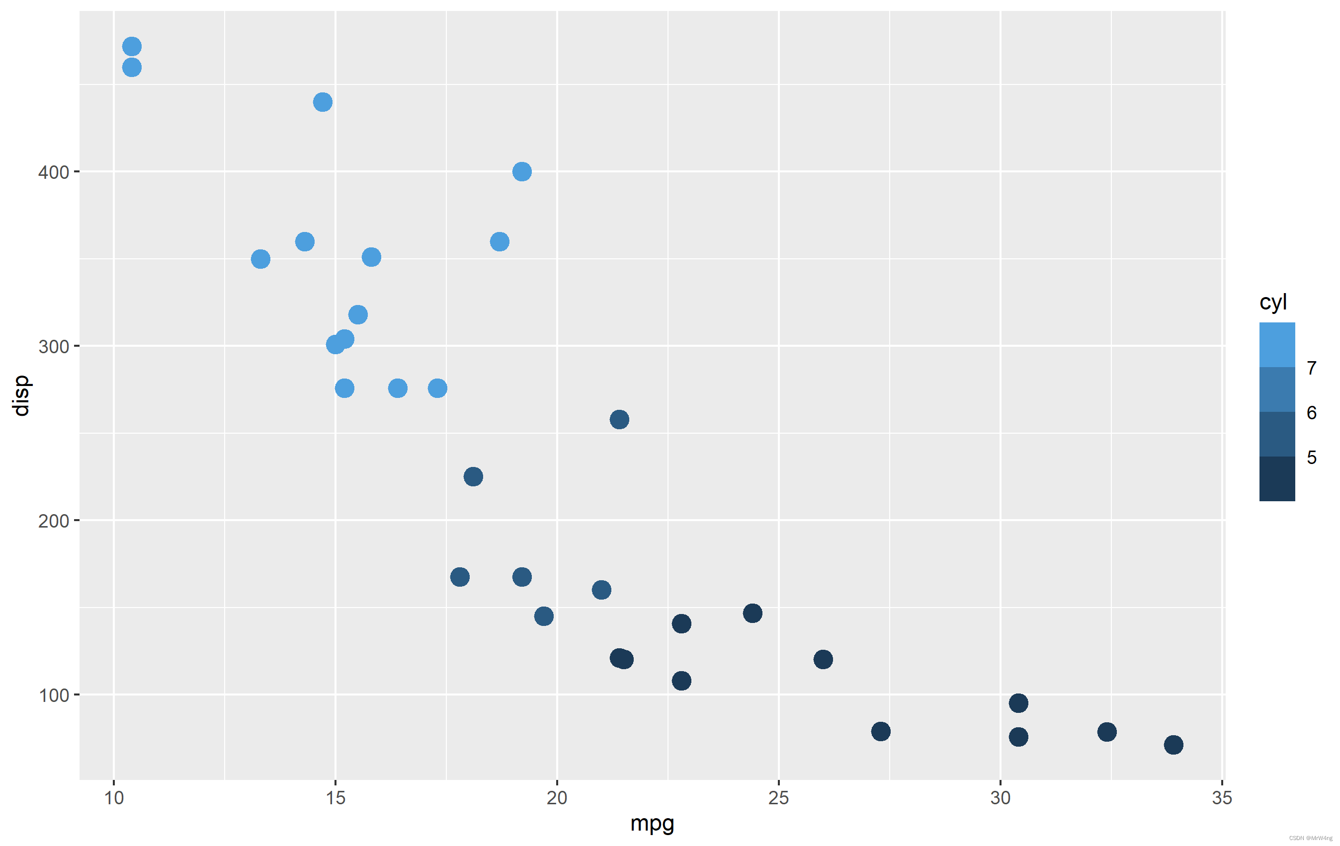
cont <- ggplot(mtcars, aes(mpg, disp, color=cyl)) + geom_point(size=4)

cont + scale_color_continuous()# scale_color_continuous可以不用添加

需要指出的是，scale_color_continuous当ggplot2检测到cyl是numeric向量后，会自动调用，为了直观，我们手动将这一函数写了出来。

在我们指定了颜色分箱之后，图例也发生了变化：

cont + scale_color_binned()

以下是连续的颜色标尺，（作用就不需要翻译了，很简单的英语，ggplot2官网也有这些函数详细的介绍）：

连续的标尺函数	颜色空间（调色板）	显示的图例	作用
scale_color_continuous()	default	Colorbar	默认
scale_color_gradient()	user-defined	Colorbar	define low and high values
scale_color_gradient2()	user-defined	Colorbar	define low mid and high values
scale_color_gradientn()	user_defined	Colorbar	define any number of incremental val
scale_color_binned()	default	Colorsteps	basic scale, but binned
scale_color_steps()	user-defined	Colorsteps	define low and high values
scale_color_steps2()	user-defined	Colorsteps	define low, mid, and high vals
scale_color_stepsn()	user-defined	Colorsteps	define any number of incremental vals
scale_color_viridis_c()	Viridis	Colorbar	viridis color scale. Change palette via option=.
scale_color_viridis_b()	Viridis	Colorsteps	Viridis color scale, binned. Change palette via option=.
scale_color_distiller()	Brewer	Colorbar	Brewer color scales. Change palette via palette=.
scale_color_fermenter()	Brewer	Colorsteps	Brewer color scale, binned. Change palette via palette=.

# 离散标尺

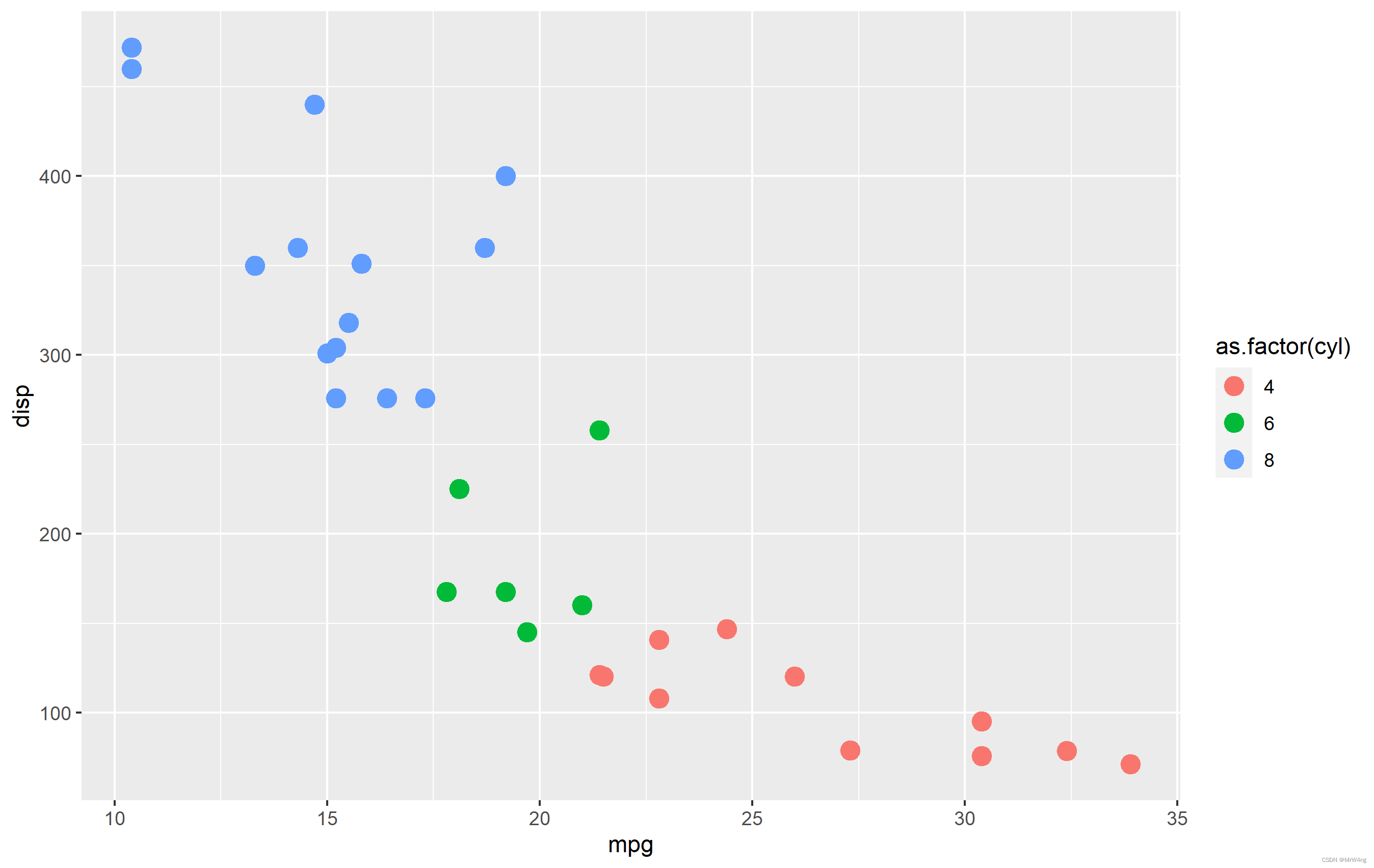
当映射数据是离散的情况下，scale_color_discrete就会被调用，同样是上面的示例，我们用as.factor函数将数值向量强行转化为因子向量后，就可以得到离散的颜色标尺。

discrete <- ggplot(mtcars, aes(mpg, disp, color=as.factor(cyl))) + geom_point(size=4)
discrete# 在这里写不写scale_color_discrete没有区别，因为它是被默认调用的

如下是有关离散的函数，如英文原文示意：

标尺函数	作用
scale_color_discrete()	默认
scale_color_hue()	Same as scale_color_discrete(), but you can define the range of hues and colors used
scale_color_grey()	Uses a greyscale. Can define the range.
scale_color_manual()	Must define specifically every color used. You can apply to your mapping by supplying a named vector for values=.
scale_color_identity()	A special-case function where your data is made up of names of colors - not names of factor levels
scale_color_brewer()	The discrete version of the Brewer colorspaces. Change palette via palette=.
scale_color_viridis_d()	The discrete version of the viridis colorspaces. Can change palette via option=.

日期标尺

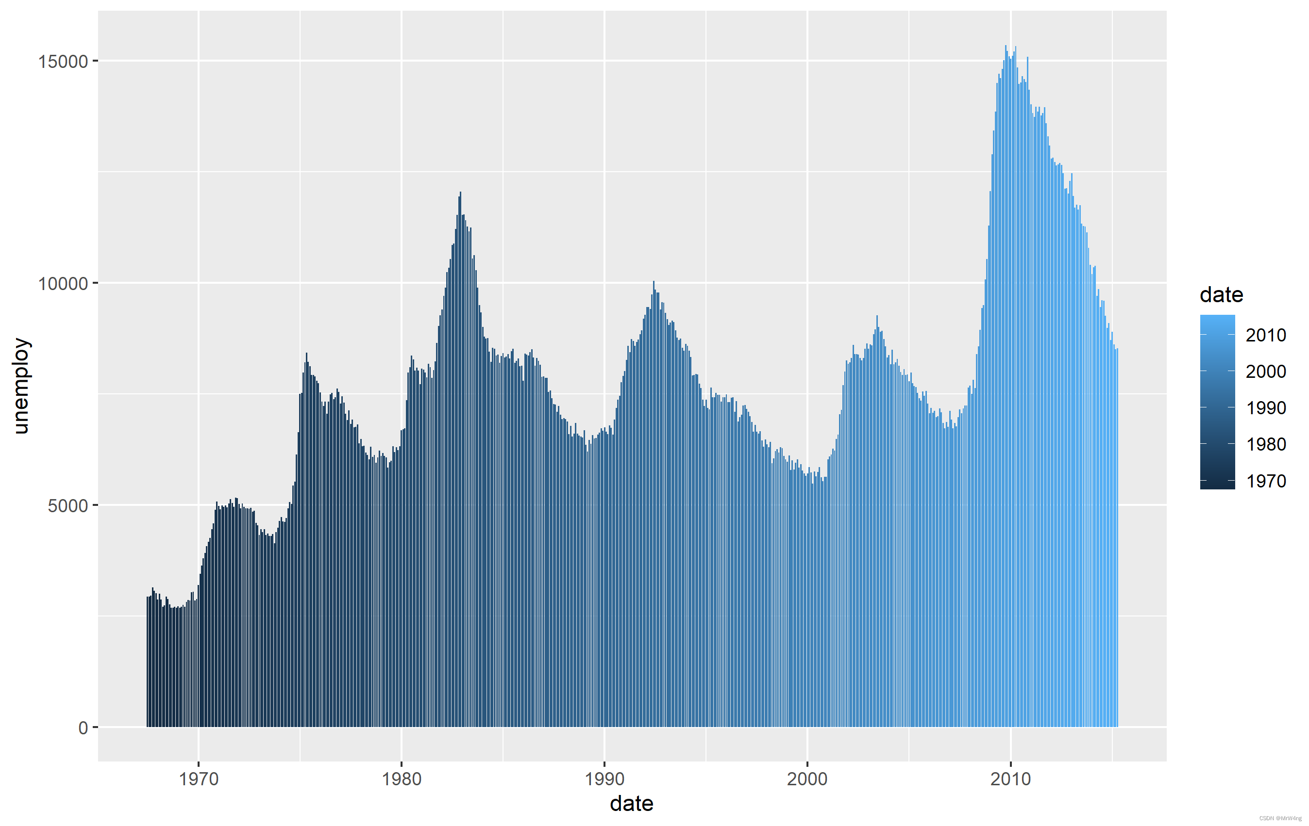
将日期映射到颜色我个人觉得是种很奇怪的行为（起码我一次都没遇到过），但既然ggplot2还是给了这种标尺（tidyverse就是喜欢重复造轮子），在文章的最后还是要介绍一下。
日期标尺主要分为scale_color_date() ，scale_color_datetime()， 顾名思义，但它们的本质和scale_color_continous没有区别，它们两都在定义函数的内部包装了scale_color_continous,使得在标签的显示上更令人易懂。

ggplot(economics, aes(x=date, y=unemploy, fill=date)) + geom_col() +scale_fill_date()

回顾曾经

如果你看到这里的话，那么下面的错误显然不用多加解释了。

> discrete + scale_color_continuous()
Error: Discrete value supplied to continuous scale

> cont + scale_color_discrete()
Error: Continuous value supplied to discrete scale