


Chapter 10
第十章
Using a Self-Organizing Map
使用自组织映射
? What is a self-organizing map (SOM)?
? Mapping colors with a SOM
? Training a SOM
? Applying the SOM to the forest cover data
This chapter focuses on using Encog to implement a self-organizing map (SOM). A SOM is a special type of neural network that classifies data. Typically, a SOM will map higher resolution data to a single or multidimensional output. This can help a neural network see the similarities among its input data. Dr. Teuvo Kohonen of the Academy of Finland created the SOM. Because of this, the SOM is sometimes called a Kohonen neural network. Encog provides two different means by which SOM networks can be trained:
本章重点介绍用encog实现自组织映射(SOM)。SOM是一种特殊的神经网络,它对数据进行分类。通常,SOM将映射更高分辨率的数据映射到单维或多维输出。这可以帮助神经网络看到输入数据之间的相似之处。芬兰书院的Teuvo Kohonen博士创建的SOM。正因为如此,SOM有时称为Kohonen神经网络。encog提供了两种SOM网络可以训练的不同方法:
? Neighborhood Competitive Training
邻域竞争培训
? Cluster Copy
集群复制
Both training types are unsupervised. This means that no ideal data is provided. The network is simply given the data and the number of categories that data should be clustered into. During training, the SOM will cluster all of the training data. Additionally, the SOM will be capable of clustering new data without retraining.
两种训练类型都是无监督的。这意味着不提供理想的数据。简单地给出了网络和数据应该被聚集到的类别的数量。在训练过程中,SOM将对所有训练数据进行聚类。此外,SOM将能够在不重新训练的情况下对新数据进行聚类。
The neighborhood competitive training method implements the classic SOM training model. The SOM is trained using a competitive, unsupervised training algorithm. Encog implements this training algorithm using the BasicTrainSOM class. This is a completely different type of training then those previously used in this book. The SOM does not use a training set or scoring object. There are no clearly defined objectives provided to the neural network at all. The only type of “objective” that the SOM has is to group similar inputs together.
邻域竞争训练法实现了经典的SOM训练模型。SOM训练使用竞争,无监督的训练算法。encog使用basictrainsom类实现这种算法。和以前在本书中使用过相比,这是一种完全不同的训练类型。SOM不使用训练集或计分对象。没有明确定义的目标提供给神经网络。SOM唯一的“目标”是将类似的输入分组在一起。
The second training type provided by Encog is a cluster copy. This is a very simple training method that simply sets the weights into a pattern to accelerate the neighborhood competitive training. This training method can also be useful with a small training set where the number of training set elements exactly matches the number of clusters. The cluster copy training method is implemented in the SOMClusterCopyTraining class.
第二种由encog提供的培训类型是集群复制。这是一种非常简单的训练方法,它只是将权重设置到一个模式里,以加速邻里的竞争训练。这种训练方法也可以用于一个小的训练集,其中训练集元素的数量正好与簇的数量相匹配。集群复制的训练方法是somclustercopytraining类实现。
The first example in this chapter will take colors as input and map similar colors together. This GUI example program will visually show how similar colors are grouped together by the self-organizing map. The output from a self-organizing map is topological. This output is usually viewed in an n-dimensional way. Often, the output is single dimensional, but it can also be two-dimensional, three-dimensional, even four-dimensional or higher. This means that the “position” of the output neurons is important. If two output neurons are closer to each other, they will be trained together more so than two neurons that are not as close.
本章的第一个示例将颜色作为输入,并将类似的颜色映射在一起。这个GUI示例程序将直观地显示自组织映射如何将相似的颜色组合在一起。自组织映射的输出是拓扑的。此输出通常以n维方式查看。通常,输出是单维的,但也可以是二维的、三维的,甚至是四维的或更高的。这意味着输出神经元的“位置”是重要的。如果两个输出神经元彼此接近,它们将一起训练,而不是两个不那么接近的神经元。
All of the neural networks that examined so far in this book have not been topological. In previous examples from this book, the distance between neurons was unimportant. Output neuron number two was just as significant to output neuron number one as was output neuron number 100.
迄今为止,在本书中所研究的所有神经网络都不是拓扑结构。在本书以前的例子中,神经元之间的距离不重要。输出神经元二号对于输出神经元一号和输出神经元数100一样重要。
10.1 The Structure and Training of a SOM
10.1 SOM的结构和训练
An Encog SOM is implemented as a two-layer neural network. The SOM simply has an input layer and an output layer. The input layer maps data to the output layer. As patterns are presented to the input layer, the output neuron with the weights most similar to the input is considered the winner.
一个encog SOM是两层的神经网络实现。SOM简单地有一个输入层和一个输出层。输入层将数据映射到输出层。当模式传入输入层,带有与输入最相似权值的输出神经元被认为是获胜者。
This similarity is calculated by comparing the Euclidean distance between eight sets of weights and the input neurons. The shortest Euclidean distance wins. Euclidean distance calculation is covered in the next section. There are no bias values in the SOM as in the feedforward neural network. Rather, there are only weights from the input layer to the output layer. Additionally, only a linear activation function is used.
这种相似性是通过比较八组权重和输入神经元之间的欧氏距离来计算的。最短欧氏距离获胜。下一节将讨论欧几里德距离计算。与前馈神经网络相比,SOM中没有偏置值。相反,只有从输入层到输出层的权重。此外,仅使用线性激活函数。
10.1.1 Structuring a SOM
10.1.1 构建SOM
We will study how to structure a SOM. This SOM will be given several colors to train on. These colors will be expressed as RGB vectors. The individual red, green and blue values can range between -1 and +1. Where -1 is no color, or black, and +1 is full intensity of red, green or blue. These three-color components comprise the neural network input.
我们将研究如何构造SOM。这个SOM将被赋予几种颜色来训练。这些颜色将用RGB向量表示。单个红色、绿色和蓝色值可以介于-1和1之间。- 1没有颜色,或黑色,1是完全强度的红色,绿色或蓝色。这三个颜色分量组成神经网络输入。
The output is a 2,500-neuron grid arranged into 50 rows by 50 columns. This SOM will organize similar colors near each other in this output grid. Figure 10.1 shows this output.
输出是一个2500个神经元网格,50列50行。这个SOM将在输出网格中组织类似的颜色。图10.1显示了这个输出。

The above figure may not be as clear in black and white editions of this book as it is in color. However, you can see similar colors grouped near each other. A single, color-based SOM is a very simple example that allows you to visualize the grouping capabilities of the SOM.
上面的图在本书的黑白版本中可能不太清楚,因为它是彩色的。不过,您可以看到类似的颜色接近对方分组。一个单一基于颜色的SOM是一个非常简单的示例,它允许您可视化SOM的分组功能。
10.1.2 Training a SOM
10.1.2 训练SOM
How is a SOM trained? The training process will update the weight matrix, which is 3 x2,500. Initialize the weight matrix to random values to start. Then 15 training colors are randomly chosen.
如何训练SOM?训练过程中,将更新3x2500的权重矩阵。将权重矩阵初始化为随机值以开始。然后随机选取15种训练颜色。
Just like previous examples, training will progress through a series of iterations. However, unlike feedforward neural networks, SOM networks are usually trained with a fixed number of iterations. For the colors example in this chapter, we will use 1,000 iterations.
就像前面的例子一样,训练将通过一系列迭代来进行。然而,与前馈神经网络不同,SOM网络通常经过一个固定数量的迭代训练。对于本章中的颜色示例,我们将使用1000个迭代。
Begin training the color sample that we wish to train for by choosing one random color sample per iteration. Pick one output neuron whose weights most closely match the basis training color. The training pattern is a vector of three numbers. The weights between each of the 2,500 output neurons and the three input neurons are also a vector of three numbers. Calculate the Euclidean distance between the weight and training pattern. Both are a vector of three numbers. This is done with Equation 10.1.
开始训练我们希望训练的颜色样本,每次迭代选择一个随机颜色样本。选择一个权值最接近基础训练色的输出神经元。训练模式是三个数字的向量。2500个输出神经元和三个输入神经元之间的权值也是三个数的向量。计算权重和训练模式之间的欧氏距离。两者都是三个数的向量。这是用方程10.1完成的。

This is very similar to Equation 2.3, shown in Chapter 2. In the above equation the variable p represents the input pattern. The variable w represents the weight vector. By squaring the differences between each vector component and taking the square root of the resulting sum, we realize the Euclidean distance. This measures how different each weight vector is from the input training pattern.
这与第2章中所示的方程式2.3非常相似。在上述等式中,变量p代表输入模式。变量w表示权向量。通过对各矢量分量之间的差平方和取所得平方的平方根,实现欧氏距离。衡量每个权重向量与输入训练模式的不同程度。
This distance is calculated for every output neuron. The output neuron with the shortest distance is called the Best Matching Unit (BMU). The BMU is the neuron that will learn the most from the training pattern. The neighbors of the BMU will learn less. Now that a BMU is determined, loop over all weights in the matrix. Update every weight according to Equation 10.2.
计算每个输出神经元的距离。最短距离的输出神经元被称为最佳匹配单元(BMU)。BMU是从训练模式学的最多的神经元。BMU的邻居学的少些。现在确定了一个BMU,遍历权重矩阵,根据等式10.2更新每一个权重。

In the above equation, the variable t represents time, or the iteration number. The purpose of the equation is to calculate the resulting weight vector Wv(t+1). The next weight will be calculated by adding to the current weight, which is Wv(t). The end goal is to calculate how different the current weight is from the input vector. The clause D(T)-Wv(t) achieves this. If we simply added this value to the weight, the weight would exactly match the input vector. We don’t want to do this. As a result, we scale it by multiplying it by two ratios. The first ratio, represented by theta, is the neighborhood function. The second ratio is a monotonically decreasing learning rate.
在上述方程中,变量t表示时间,或迭代次数。该方程的目的是计算得到的权重向量WV(T + 1)。接下来的权重会增加当前权重Wv(t)。最终目标是计算当前权重与输入向量的不同。语句D(T)- WV(T)达到此目的。如果我们简单地将这个值添加到权重,权重将正好匹配输入向量。我们不想这样做。我们把它乘以两个比例。以θ表示的第一个比率是邻域函数。第二个比率是单调递减的学习率。
The neighborhood function considers how close the output neuron we are training is to the BMU. For closer neurons, the neighborhood function will be close to one. For distant neighbors the neighborhood function will return zero.This controls how near and far neighbors are trained.
邻域函数考虑我们正训练的输出神经元是多么接近BMU。对于更近的神经元,邻近函数将接近一。对于遥远的邻居,邻域函数将返回零。这就控制了远近邻居如何训练。
We will look at how the neighborhood function determines this in the next section. The learning rate also scales how much the output neuron will learn. This learning rate is similar to the learning rate used in backpropagation training. However, the learning rate should decrease as the training progresses.
我们将在下一节中看看邻域函数是如何确定的。输出神经元将学习学习率还可以缩放多少。这种学习速率类似于反向传播训练中使用的学习速率。然而,随着训练的进展,学习率会下降。
This learning rate must decrease monotonically, meaning the function output only decreases or remains the same as time progresses. The output from the function will never increase at any interval as time increases.
这个学习率必须递减,这意味着函数输出只会随着时间的推移而减少或保持不变。随着时间的增加,函数的输出在任何时间间隔都不会增加。
10.1.3 Understanding Neighborhood Functions
10.1.3 了解邻域函数
The neighborhood function determines to what degree each output neuron should receive training from the current training pattern. The neighborhood function will return a value of one for the BMU. This indicates that it should receive the most training of any neurons. Neurons further from the BMU will receive less training. The neighborhood function determines this percent.
邻域函数决定了每个输出神经元从当前训练模式接受训练的程度。邻域函数将为BMU返回值。这表明它应该接受最多的神经元训练。离BMU较远的神经元将获得较少的训练。邻域函数决定这个百分比。
If the output is arranged in only one dimension, a simple one-dimensional neighborhood function should be used. A single dimension self-organizing map treats the output as one long array of numbers. For instance, a single dimension network might have 100 output neurons that are simply treated as a long, single dimension array of 100 values.
如果输出仅在一个维度中排列,则应使用一个简单的一维邻域函数。一维自组织映射将输出视为一长串数字。例如,一个一维网络可能有100个输出神经元,这些神经元被简单地看作是一个长的、一维的100个值数组。
A two-dimensional SOM might take these same 100 values and treat them as a grid, perhaps of 10 rows and 10 columns. The actual structure remains the same; the neural network has 100 output neurons. The only difference is the neighborhood function. The first would use a single dimensional neighborhood function; the second would use a two-dimensional neighborhood function. The function must consider this additional dimension and factor it into the distance returned.
一个二维SOM可能采用相同的100个值,并把它们当作网格,可能是10行10列。实际结构保持不变,神经网络有100个输出神经元。唯一的区别是邻域函数。第一种使用一维邻域函数,第二种使用二维邻域函数。函数必须考虑这个附加维度,并将其添加到返回的距离中。
It is also possible to have three, four, and even more dimensional functions for the neighborhood function. Two-dimension is the most popular choice. Single dimensional neighborhood functions are also somewhat common. Three or more dimensions are more unusual. It really comes down to computing how many ways an output neuron can be close to another. Encog supports any number of dimensions, though each additional dimension adds greatly to the amount of memory and processing power needed.
也有可能有三,四,甚至更多的维函数的邻域函数。二维是最流行的选择。一维邻域函数也有点常见。三个或更多维度不经常使用。这实际上取决于计算输出神经元能接近多少种方法。encog支持任何维,虽然每一个额外的维数大大增加了需要的内存和处理能力。
The Gaussian function is a popular choice for a neighborhood function. The Gaussian function has single- and multi-dimensional forms. The singledimension Gaussian function is shown in Equation 10.3.
高斯函数是邻域函数的常用选择。高斯函数具有单维和多维形式。单维度高斯函数公式10.3所示。

The graph of the Gaussian function is shown in Figure 10.2.
高斯函数的图如图10.2所示。

The above figure shows why the Gaussian function is a popular choice for a neighborhood function. If the current output neuron is the BMU, then its distance (x-axis) will be zero. As a result, the training percent (y-axis) is 100%. As the distance increases either positively or negatively, the training percentage decreases. Once the distance is great enough, the training percent is near zero.
上面的图说明为什么高斯函数是邻域函数的常用选择。如果当前的输出神经元是BMU,那么它的距离(X轴)将为零。因此,训练百分比(y轴)是100%。随着距离的增加,无论是正的还是负的,训练百分比都会降低。一旦距离足够大,训练百分比接近零。
There are several constants in Equation 10.3 that govern the shape of the Gaussian function. The constants a is the height of the curve’s peak, b is the position of the center of the peak, and c constants the width of the ”bell”. The variable x represents the distance that the current neuron is from the BMU. The above Gaussian function is only useful for a one-dimensional output array. If using a two-dimensional output grid, it is important to use the twodimensional form of the Gaussian function. Equation 10.4 shows this.
在方程10.3中有几个常数来控制高斯函数的形状。常数a是曲线峰的高度,b是峰的中心位置,c常数是“铃”的宽度。变量x代表当前神经元与BMU的距离。上述高斯函数只适用于一维输出阵列。如果使用二维输出网格,应使用高斯函数的二维形式。方程式10.4显示了这一点。

The graph form of the two-dimensional form of the Gaussian function is shown
in Figure 10.3.
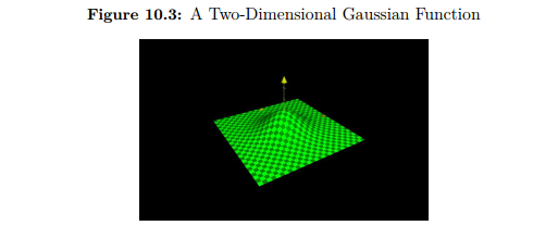
The two-dimensional form of the Gaussian function takes a single peak variable, but allows the user to specify separate values for the position and width of the curve. The equation does not need to be symmetrical.
高斯函数的二维形式采用单峰变量,但允许用户为曲线的位置和宽度指定单独的值。这个方程不需要是对称的。
How are the Gaussian constants used with a neural network? The peak is almost always one. To unilaterally decrease the effectiveness of training, the peak should be set below one. However, this is more the role of the learning rate. The center is almost always zero to center the curve on the origin. If the center is changed, then a neuron other than the BMU would receive the full learning. It is unlikely you would ever want to do this. For a multi-dimensional Gaussian, set all centers to zero to truly center the curve at the origin.
高斯常数如何与神经网络一起使用?尖峰几乎总是一个。为单方面降低训练效果,应将峰值设置在1以下。然而,这更重要的是学习率的作用。中心几乎总是零,使曲线在原点上居中。如果中心发生了改变,那么神经元除了BMU会得到充分的学习。你一般不会这样做。对于多维高斯,将所有的中心设为零以便真正的曲线中心在原点处。
This leaves the width of the Gaussian function. The width should be set to something slightly less than the entire width of the grid or array. Then the width should be gradually decreased. The width should be decreased monotonically just like the learning rate.
这就留下了高斯函数的宽度。宽度应该设置为略小于网格或数组的整个宽度。宽度应逐渐减小。宽度应像学习速率一样单调递减。
10.1.4 Forcing a Winner
10.1.4 强制一个赢家
An optional feature to Encog SOM competitive training is the ability to force a winner. By default, Encog does not force a winner. However, this feature can be enabled for SOM training. Forcing a winner will try to ensure that each output neuron is winning for at least one of the training samples. This can cause a more even distribution of winners. However, it can also skew the data as somewhat “engineers” the neural network. Because of this, it is disabled by default.
对encog SOM竞技训练的一个可选功能是迫使赢家的能力。默认情况下,Encog没有强制一个赢家。但是,这个特性可以用于SOM训练。强迫一个胜利者将尝试确保每个输出神经元至少为一个训练样本获胜。这可能导致优胜者更均匀地分配。然而,它也可以将数据扭曲为某种“工程师”的神经网络。因此,默认情况下它是禁用的。
10.1.5 Calculating Error
10.1.5 计算误差
In propagation training we could measure the success of our training by examining the neural network current error. In a SOM there is no direct error because there is no expected output. Yet, the Encog interface Train exposes an error property. This property does return an estimation of the SOM error.
在传播训练中,我们可以通过检测神经网络当前误差来衡量训练的成功。在SOM中没有直接的错误,因为没有预期的输出。然而,这encog接口Train暴露误差特性。此属性确实返回SOM错误的估计值。
The error is defined to be the ”worst” or longest Euclidean distance of any BMUs. This value should be minimized as learning progresses. This gives a general approximation of how well the SOM has been trained.
误差被定义为“坏的”或与任何BMUs的长距离。随着学习的进展,这个值应该最小化。这就给出了SOM训练的一般近似值。
10.2 Implementing the Colors SOM in Encog
10.2 使用Encog实现颜色SOM
We will now see how the color matching SOM is implemented. There are two classes that make up this example:
现在我们将了解如何实现颜色匹配SOM。这个例子有两个类:
? MapPanel
? SomColors
The MapPanel class is used to display the weight matrix to the screen. The SomColors class extends the JPanel class and adds the MapPanel to itself for display. We will examine both classes, starting with the MapPanel.
mappanel类用于显示权重矩阵屏幕。somcolors类扩展JPanel类增加mappanel本身显示。我们将研究这两个类,从mappanel开始。
10.2.1 Displaying the Weight Matrix
10.2.1 展示权重矩阵
The MapPanel class draws the GUI display for the SOM as it progresses. This relatively simple class can be found at the following location.
类mappanel绘制GUI显示SOM的进展。这个相对简单的类可以在下面的位置找到。
org.encog.examples.neural.gui.som.MapPanel
The convertColor function is very important. It converts a double that contains a range of -1 to +1 into the 0 to 255 range that an RGB component requires. A neural network deals much better with -1 to +1 than 0 to 255. As a result, this normalization is needed.
convertcolor功能是非常重要的。它将包含1 - 1范围的double转换为RGB分量所需的0到255范围。一个神经网络处理—1到1比0到255要好得多。因此,需要进行这种规范化。
private int convertColor (double d ) {
double result = 128*d ;
result +=128;
result = Math.min ( result , 255) ;
result = Math.max( result , 0) ;
return ( int ) result ;
}
The number 128 is the midpoint between 0 and 255. We multiply the result by 128 to get it to the proper range and then add 128 to diverge from the midpoint. This ensures that the result is in the proper range.
数字128是0和255之间的中点。我们把结果乘以128,使其达到适当的范围,然后从中点加上128。这样可以确保结果在适当的范围内。
Using the convertColor method the paint method can properly draw the state of the SOM. The output from this function will be a color map of all of the neural network weights. Each of the 2,500 output neurons is shown on a grid. Their color is determined by the weight between that output neuron and the three input neurons. These three weights are treated as RGB color components. The convertColor method is shown here.
使用方法convertcolor绘制方法可以画出SOM的状态。该函数的输出将是所有神经网络权值的颜色映射。2500个输出神经元中的每一个都显示在网格上。它们的颜色取决于输出神经元和三个输入神经元之间的权重。这三个权重被视为RGB颜色分量。convertcolor方法如下所示。
public void paint ( Graphics g )
{
Begin by looping through all 50 rows and columns.
for ( int y = 0 ; y< HEIGHT; y++) {
for ( int x = 0 ; x< WIDTH; x++) {
While the output neurons are shown as a two-dimensional grid, they are all stored as a one-dimensional array. We must calculate the current onedimensional index from the two-dimensional x and y values.
当输出神经元被显示为二维网格时,它们都被存储为一维数组。我们必须从二维的X和Y值计算当前一维位置。
int index = ( y?WIDTH)+x ;
We obtain the three weight values from the matrix and use the convertColor method to convert these to RGB components.
int red = convertColor ( weights.get ( 0 , index ) ) ;
int green = convertColor ( weights.get ( 1 , index ) ) ;
int blue = convertColor ( weights.get ( 2 , index ) ) ;
These three components are used to create a new Color object.
g.setColor (new Color ( red , green , blue ) ) ;
A filled rectangle is displayed to display the neuron.
g.fillRect( x?CELL SIZE , y?CELL SIZE , CELL SIZE , CELL SIZE) ;
}
}
}
Once the loops complete, the entire weight matrix has been displayed to the screen.
一旦循环完成,整个权重矩阵就显示在屏幕上。
10.2.2 Training the Color Matching SOM
10.2.2 训练颜色匹配SOM
The SomColors class acts as the main JPanel for the application. It also provides the neural network all of the training. This class can be found at the following location.
应用程序中somcolors类主要作为JPanel使用。它还提供了所有训练的神经网络。可以在以下位置找到此类。
package org.encog.examples.neural.gui.som.SomColors
The BasicTrainSOM class must be set up so that the neural network will train. To do so, a neighborhood function is required. For this example, use the NeighborhoodGaussian neighborhood function. This neighborhood function can support a multi-dimensional Gaussian neighborhood function. The following line of code creates this neighborhood function.
basictrainsom类必须建立以便神经网络训练。为此,需要一个邻域函数。在这个例子中,使用neighborhoodgaussian邻域函数。这个邻域函数可以支持多维高斯邻域函数。下面的代码行创建了这个邻域函数。
this.gaussian = new NeighborhoodRBF (RBFEnum.Gaussian , MapPanel.WIDTH, MapPanel.HEIGHT) ;
This constructor creates a two-dimensional Gaussian neighborhood function. The first two parameters specify the height and width of the grid. There are other constructors that can create higher dimensional Gaussian functions. Additionally, there are other neighborhood functions provided by Encog. The most common is the NeighborhoodRBF. NeighborhoodRBF can use a Gaussian, or other radial basis functions. Below is the complete list of neighborhood functions.
这个构造函数创建一个二维高斯邻域函数。前两个参数指定网格的高度和宽度。还有其他构造函数可以创建更高维的高斯函数。此外,还有由encog提供的其他邻域函数。最常见的是neighborhoodrbf。neighborhoodrbf可以使用高斯或其他径向基函数。下面是邻域函数的完整列表。
? NeighborhoodBubble
? NeighborhoodRBF
? NeighborhoodRBF1D
? NeighborhoodSingle
The NeighborhoodBubble only provides one-dimensional neighborhood functions. A radius is specified and anything within that radius receives full training. The NeighborhoodSingle functions as a single-dimensional neighborhood function and only allows the BMU to receive training.
neighborhoodbubble只提供一维邻域函数。指定半径,半径内的任何物体都接受完全的训练。neighborhoodsingle功能作为一个单维邻域函数和只允许BMU接受培训。
The NeighborhoodRBF class supports several RBF functions. The ”Mexican Hat” and ”Gaussian” RBF’s are common choices. However the Multiquadric and the Inverse Multiquadric are also available. We must also create a CompetitiveTraining object to make use of the neighborhood function.
neighborhoodrbf类支持几种RBF函数。“墨西哥帽”和“高斯”的RBF是常见的选择。然而,二次函数和逆二次函数也可。我们还必须创造一个competitivetraining对象利用邻域函数。
this.train = new BasicTrainSOM ( this.network , 0.01 , null , gaussian );
The first parameter specifies the network to train and the second parameter is the learning rate. Automatically decrease the learning rate from a maximum value to a minimum value, so the learning rate specified here is not important.
第一个参数指定要训练的网络,第二个参数是学习速率。自动将学习速率从最大值降到最小值,因此这里指定的学习速率不重要。
The third parameter is the training set. Randomly feed colors to the neural network, thus eliminating the need for the training set. Finally, the fourth parameter is the newly created neighborhood function.
第三个参数是训练集。随机给神经网络提供颜色,从而消除了训练集的需要。最后,第四个参数是新创建的邻域函数。
The SOM training is provided for this example by a background thread. This allows the training to progress while the user watches. The background thread is implemented in the run method, as shown here.
通过后台线程为这个示例提供SOM培训。这使得培训可以在用户观看时进行。后台线程是在run方法中实现的,如下所示。
public void run ( ) {
The run method begins by creating the 15 random colors to train the neural network. These random samples will be stored in the samples variable, which is a List.
List<MLData> samples = new ArrayList<MLData>() ;
The random colors are generated and have random numbers for the RGB components.
for ( int i =0; i <15; i++) {
MLData data = new BasicMLData (3) ;
data.setData (0 , RangeRandomizer.randomize ( -1 ,1) ) ;
data.setData (1 , RangeRandomizer.randomize ( -1 ,1) ) ;
data.setData (2 , RangeRandomizer.randomize ( -1 ,1) ) ;
samples.add( data ) ;
}
The following line sets the parameters for the automatic decay of the learning rate and the radius.
this.train.setAutoDecay (1000 , 0.8 , 0.003 , 30 , 5) ;
We must provide the anticipated number of iterations. For this example, the quantity is 1,000. For SOM neural networks, it is necessary to know the number of iterations up front. This is different than propagation training that trained for either a specific amount of time or until below a specific error rate.
我们必须提供预期的迭代次数。对于这个例子,数量是1000。对于SOM神经网络,有必要知道前面的迭代次数。这与传播训练不同,传播训练或是指定训练时间,或是低于特定错误率。
The parameters 0.8 and 0.003 are the beginning and ending learning rates. The error rate will be uniformly decreased from 0.8 to 0.003 over each iteration. It should reach close to 0.003 by the last iteration.
参数0.8和0.003是开始和结束学习率。每次迭代时,错误率将均匀地从0.8下降到0.003。在最后一次迭代中它应该接近0.003。
Likewise, the parameters 30 and 5 represent the beginning and ending radius. The radius will start at 30 and should be near 5 by the final iteration. If more than the planned 1,000 iterations are performed, the radius and learning rate will not fall below their minimums.
同样,参数30和5表示开始和结束半径。半径将从30开始,到最后迭代时将接近5。如果超过计划1000进行迭代,半径和学习率不会低于最小值。
for ( int i =0; i <1000; i++) {
For each competitive learning iteration, there are two choices. First, you can choose to simply provide an MLDataSet that contains the training data and call the iteration method CompetitiveTraining. Next we choose a random color index and obtain that color.
对于每一个竞争学习迭代,有两种选择。首先,你可以选择简单地提供一个mldataset包含训练数据和调用迭代法competitivetraining。接下来,我们选择一个随机颜色索引并获得该颜色。
int idx = ( int ) (Math.random ( ) ? samples.s i z e ( ) ) ;
MLData c = samples.get ( idx ) ;
The trainPattern method will train the neural network for this random color pattern. The BMU will be located and updated as described earlier in this chapter.
trainpattern方法将训练这个随机颜色模式的神经网络。象本章前面介绍的那样,BMU将被确定和更新。
this.train.trainPattern ( c ) ;
Alternatively, the colors could have been loaded into an MLDataSet object and the iteration method could have been used. However, training the patterns one at a time and using a random pattern looks better when displayed on the screen. Next, call the autoDecay method to decrease the learning rate and radius according to the parameters previously specified.
另外,颜色可以被加载到一个mldataset对象和迭代方法可能被使用。然而,在屏幕上显示时,一次使用一个模式并使用一个随机模式看起来更好。接下来,根据预先指定的参数调用autodecay方法降低学习速度和半径。
this.train.autoDecay ( ) ;
The screen is repainted.
this.map.repaint ( ) ;
Finally, we display information about the current iteration.
System.out.println ( ”Iteration” + i + ” , ”
+ this.train.toString() ) ;
}
}
This process continues for 1,000 iterations. By the final iteration, the colors will be grouped.
此过程持续1000次迭代。通过最后的迭代,颜色将被分组。
第十章
Using a Self-Organizing Map
使用自组织映射
? What is a self-organizing map (SOM)?
? Mapping colors with a SOM
? Training a SOM
? Applying the SOM to the forest cover data
This chapter focuses on using Encog to implement a self-organizing map (SOM). A SOM is a special type of neural network that classifies data. Typically, a SOM will map higher resolution data to a single or multidimensional output. This can help a neural network see the similarities among its input data. Dr. Teuvo Kohonen of the Academy of Finland created the SOM. Because of this, the SOM is sometimes called a Kohonen neural network. Encog provides two different means by which SOM networks can be trained:
本章重点介绍用encog实现自组织映射(SOM)。SOM是一种特殊的神经网络,它对数据进行分类。通常,SOM将映射更高分辨率的数据映射到单维或多维输出。这可以帮助神经网络看到输入数据之间的相似之处。芬兰书院的Teuvo Kohonen博士创建的SOM。正因为如此,SOM有时称为Kohonen神经网络。encog提供了两种SOM网络可以训练的不同方法:
? Neighborhood Competitive Training
邻域竞争培训
? Cluster Copy
集群复制
Both training types are unsupervised. This means that no ideal data is provided. The network is simply given the data and the number of categories that data should be clustered into. During training, the SOM will cluster all of the training data. Additionally, the SOM will be capable of clustering new data without retraining.
两种训练类型都是无监督的。这意味着不提供理想的数据。简单地给出了网络和数据应该被聚集到的类别的数量。在训练过程中,SOM将对所有训练数据进行聚类。此外,SOM将能够在不重新训练的情况下对新数据进行聚类。
The neighborhood competitive training method implements the classic SOM training model. The SOM is trained using a competitive, unsupervised training algorithm. Encog implements this training algorithm using the BasicTrainSOM class. This is a completely different type of training then those previously used in this book. The SOM does not use a training set or scoring object. There are no clearly defined objectives provided to the neural network at all. The only type of “objective” that the SOM has is to group similar inputs together.
邻域竞争训练法实现了经典的SOM训练模型。SOM训练使用竞争,无监督的训练算法。encog使用basictrainsom类实现这种算法。和以前在本书中使用过相比,这是一种完全不同的训练类型。SOM不使用训练集或计分对象。没有明确定义的目标提供给神经网络。SOM唯一的“目标”是将类似的输入分组在一起。
The second training type provided by Encog is a cluster copy. This is a very simple training method that simply sets the weights into a pattern to accelerate the neighborhood competitive training. This training method can also be useful with a small training set where the number of training set elements exactly matches the number of clusters. The cluster copy training method is implemented in the SOMClusterCopyTraining class.
第二种由encog提供的培训类型是集群复制。这是一种非常简单的训练方法,它只是将权重设置到一个模式里,以加速邻里的竞争训练。这种训练方法也可以用于一个小的训练集,其中训练集元素的数量正好与簇的数量相匹配。集群复制的训练方法是somclustercopytraining类实现。
The first example in this chapter will take colors as input and map similar colors together. This GUI example program will visually show how similar colors are grouped together by the self-organizing map. The output from a self-organizing map is topological. This output is usually viewed in an n-dimensional way. Often, the output is single dimensional, but it can also be two-dimensional, three-dimensional, even four-dimensional or higher. This means that the “position” of the output neurons is important. If two output neurons are closer to each other, they will be trained together more so than two neurons that are not as close.
本章的第一个示例将颜色作为输入,并将类似的颜色映射在一起。这个GUI示例程序将直观地显示自组织映射如何将相似的颜色组合在一起。自组织映射的输出是拓扑的。此输出通常以n维方式查看。通常,输出是单维的,但也可以是二维的、三维的,甚至是四维的或更高的。这意味着输出神经元的“位置”是重要的。如果两个输出神经元彼此接近,它们将一起训练,而不是两个不那么接近的神经元。
All of the neural networks that examined so far in this book have not been topological. In previous examples from this book, the distance between neurons was unimportant. Output neuron number two was just as significant to output neuron number one as was output neuron number 100.
迄今为止,在本书中所研究的所有神经网络都不是拓扑结构。在本书以前的例子中,神经元之间的距离不重要。输出神经元二号对于输出神经元一号和输出神经元数100一样重要。
10.1 The Structure and Training of a SOM
10.1 SOM的结构和训练
An Encog SOM is implemented as a two-layer neural network. The SOM simply has an input layer and an output layer. The input layer maps data to the output layer. As patterns are presented to the input layer, the output neuron with the weights most similar to the input is considered the winner.
一个encog SOM是两层的神经网络实现。SOM简单地有一个输入层和一个输出层。输入层将数据映射到输出层。当模式传入输入层,带有与输入最相似权值的输出神经元被认为是获胜者。
This similarity is calculated by comparing the Euclidean distance between eight sets of weights and the input neurons. The shortest Euclidean distance wins. Euclidean distance calculation is covered in the next section. There are no bias values in the SOM as in the feedforward neural network. Rather, there are only weights from the input layer to the output layer. Additionally, only a linear activation function is used.
这种相似性是通过比较八组权重和输入神经元之间的欧氏距离来计算的。最短欧氏距离获胜。下一节将讨论欧几里德距离计算。与前馈神经网络相比,SOM中没有偏置值。相反,只有从输入层到输出层的权重。此外,仅使用线性激活函数。
10.1.1 Structuring a SOM
10.1.1 构建SOM
We will study how to structure a SOM. This SOM will be given several colors to train on. These colors will be expressed as RGB vectors. The individual red, green and blue values can range between -1 and +1. Where -1 is no color, or black, and +1 is full intensity of red, green or blue. These three-color components comprise the neural network input.
我们将研究如何构造SOM。这个SOM将被赋予几种颜色来训练。这些颜色将用RGB向量表示。单个红色、绿色和蓝色值可以介于-1和1之间。- 1没有颜色,或黑色,1是完全强度的红色,绿色或蓝色。这三个颜色分量组成神经网络输入。
The output is a 2,500-neuron grid arranged into 50 rows by 50 columns. This SOM will organize similar colors near each other in this output grid. Figure 10.1 shows this output.
输出是一个2500个神经元网格,50列50行。这个SOM将在输出网格中组织类似的颜色。图10.1显示了这个输出。
The above figure may not be as clear in black and white editions of this book as it is in color. However, you can see similar colors grouped near each other. A single, color-based SOM is a very simple example that allows you to visualize the grouping capabilities of the SOM.
上面的图在本书的黑白版本中可能不太清楚,因为它是彩色的。不过,您可以看到类似的颜色接近对方分组。一个单一基于颜色的SOM是一个非常简单的示例,它允许您可视化SOM的分组功能。
10.1.2 Training a SOM
10.1.2 训练SOM
How is a SOM trained? The training process will update the weight matrix, which is 3 x2,500. Initialize the weight matrix to random values to start. Then 15 training colors are randomly chosen.
如何训练SOM?训练过程中,将更新3x2500的权重矩阵。将权重矩阵初始化为随机值以开始。然后随机选取15种训练颜色。
Just like previous examples, training will progress through a series of iterations. However, unlike feedforward neural networks, SOM networks are usually trained with a fixed number of iterations. For the colors example in this chapter, we will use 1,000 iterations.
就像前面的例子一样,训练将通过一系列迭代来进行。然而,与前馈神经网络不同,SOM网络通常经过一个固定数量的迭代训练。对于本章中的颜色示例,我们将使用1000个迭代。
Begin training the color sample that we wish to train for by choosing one random color sample per iteration. Pick one output neuron whose weights most closely match the basis training color. The training pattern is a vector of three numbers. The weights between each of the 2,500 output neurons and the three input neurons are also a vector of three numbers. Calculate the Euclidean distance between the weight and training pattern. Both are a vector of three numbers. This is done with Equation 10.1.
开始训练我们希望训练的颜色样本,每次迭代选择一个随机颜色样本。选择一个权值最接近基础训练色的输出神经元。训练模式是三个数字的向量。2500个输出神经元和三个输入神经元之间的权值也是三个数的向量。计算权重和训练模式之间的欧氏距离。两者都是三个数的向量。这是用方程10.1完成的。
This is very similar to Equation 2.3, shown in Chapter 2. In the above equation the variable p represents the input pattern. The variable w represents the weight vector. By squaring the differences between each vector component and taking the square root of the resulting sum, we realize the Euclidean distance. This measures how different each weight vector is from the input training pattern.
这与第2章中所示的方程式2.3非常相似。在上述等式中,变量p代表输入模式。变量w表示权向量。通过对各矢量分量之间的差平方和取所得平方的平方根,实现欧氏距离。衡量每个权重向量与输入训练模式的不同程度。
This distance is calculated for every output neuron. The output neuron with the shortest distance is called the Best Matching Unit (BMU). The BMU is the neuron that will learn the most from the training pattern. The neighbors of the BMU will learn less. Now that a BMU is determined, loop over all weights in the matrix. Update every weight according to Equation 10.2.
计算每个输出神经元的距离。最短距离的输出神经元被称为最佳匹配单元(BMU)。BMU是从训练模式学的最多的神经元。BMU的邻居学的少些。现在确定了一个BMU,遍历权重矩阵,根据等式10.2更新每一个权重。
In the above equation, the variable t represents time, or the iteration number. The purpose of the equation is to calculate the resulting weight vector Wv(t+1). The next weight will be calculated by adding to the current weight, which is Wv(t). The end goal is to calculate how different the current weight is from the input vector. The clause D(T)-Wv(t) achieves this. If we simply added this value to the weight, the weight would exactly match the input vector. We don’t want to do this. As a result, we scale it by multiplying it by two ratios. The first ratio, represented by theta, is the neighborhood function. The second ratio is a monotonically decreasing learning rate.
在上述方程中,变量t表示时间,或迭代次数。该方程的目的是计算得到的权重向量WV(T + 1)。接下来的权重会增加当前权重Wv(t)。最终目标是计算当前权重与输入向量的不同。语句D(T)- WV(T)达到此目的。如果我们简单地将这个值添加到权重,权重将正好匹配输入向量。我们不想这样做。我们把它乘以两个比例。以θ表示的第一个比率是邻域函数。第二个比率是单调递减的学习率。
The neighborhood function considers how close the output neuron we are training is to the BMU. For closer neurons, the neighborhood function will be close to one. For distant neighbors the neighborhood function will return zero.This controls how near and far neighbors are trained.
邻域函数考虑我们正训练的输出神经元是多么接近BMU。对于更近的神经元,邻近函数将接近一。对于遥远的邻居,邻域函数将返回零。这就控制了远近邻居如何训练。
We will look at how the neighborhood function determines this in the next section. The learning rate also scales how much the output neuron will learn. This learning rate is similar to the learning rate used in backpropagation training. However, the learning rate should decrease as the training progresses.
我们将在下一节中看看邻域函数是如何确定的。输出神经元将学习学习率还可以缩放多少。这种学习速率类似于反向传播训练中使用的学习速率。然而,随着训练的进展,学习率会下降。
This learning rate must decrease monotonically, meaning the function output only decreases or remains the same as time progresses. The output from the function will never increase at any interval as time increases.
这个学习率必须递减,这意味着函数输出只会随着时间的推移而减少或保持不变。随着时间的增加,函数的输出在任何时间间隔都不会增加。
10.1.3 Understanding Neighborhood Functions
10.1.3 了解邻域函数
The neighborhood function determines to what degree each output neuron should receive training from the current training pattern. The neighborhood function will return a value of one for the BMU. This indicates that it should receive the most training of any neurons. Neurons further from the BMU will receive less training. The neighborhood function determines this percent.
邻域函数决定了每个输出神经元从当前训练模式接受训练的程度。邻域函数将为BMU返回值。这表明它应该接受最多的神经元训练。离BMU较远的神经元将获得较少的训练。邻域函数决定这个百分比。
If the output is arranged in only one dimension, a simple one-dimensional neighborhood function should be used. A single dimension self-organizing map treats the output as one long array of numbers. For instance, a single dimension network might have 100 output neurons that are simply treated as a long, single dimension array of 100 values.
如果输出仅在一个维度中排列,则应使用一个简单的一维邻域函数。一维自组织映射将输出视为一长串数字。例如,一个一维网络可能有100个输出神经元,这些神经元被简单地看作是一个长的、一维的100个值数组。
A two-dimensional SOM might take these same 100 values and treat them as a grid, perhaps of 10 rows and 10 columns. The actual structure remains the same; the neural network has 100 output neurons. The only difference is the neighborhood function. The first would use a single dimensional neighborhood function; the second would use a two-dimensional neighborhood function. The function must consider this additional dimension and factor it into the distance returned.
一个二维SOM可能采用相同的100个值,并把它们当作网格,可能是10行10列。实际结构保持不变,神经网络有100个输出神经元。唯一的区别是邻域函数。第一种使用一维邻域函数,第二种使用二维邻域函数。函数必须考虑这个附加维度,并将其添加到返回的距离中。
It is also possible to have three, four, and even more dimensional functions for the neighborhood function. Two-dimension is the most popular choice. Single dimensional neighborhood functions are also somewhat common. Three or more dimensions are more unusual. It really comes down to computing how many ways an output neuron can be close to another. Encog supports any number of dimensions, though each additional dimension adds greatly to the amount of memory and processing power needed.
也有可能有三,四,甚至更多的维函数的邻域函数。二维是最流行的选择。一维邻域函数也有点常见。三个或更多维度不经常使用。这实际上取决于计算输出神经元能接近多少种方法。encog支持任何维,虽然每一个额外的维数大大增加了需要的内存和处理能力。
The Gaussian function is a popular choice for a neighborhood function. The Gaussian function has single- and multi-dimensional forms. The singledimension Gaussian function is shown in Equation 10.3.
高斯函数是邻域函数的常用选择。高斯函数具有单维和多维形式。单维度高斯函数公式10.3所示。
The graph of the Gaussian function is shown in Figure 10.2.
高斯函数的图如图10.2所示。
The above figure shows why the Gaussian function is a popular choice for a neighborhood function. If the current output neuron is the BMU, then its distance (x-axis) will be zero. As a result, the training percent (y-axis) is 100%. As the distance increases either positively or negatively, the training percentage decreases. Once the distance is great enough, the training percent is near zero.
上面的图说明为什么高斯函数是邻域函数的常用选择。如果当前的输出神经元是BMU,那么它的距离(X轴)将为零。因此,训练百分比(y轴)是100%。随着距离的增加,无论是正的还是负的,训练百分比都会降低。一旦距离足够大,训练百分比接近零。
There are several constants in Equation 10.3 that govern the shape of the Gaussian function. The constants a is the height of the curve’s peak, b is the position of the center of the peak, and c constants the width of the ”bell”. The variable x represents the distance that the current neuron is from the BMU. The above Gaussian function is only useful for a one-dimensional output array. If using a two-dimensional output grid, it is important to use the twodimensional form of the Gaussian function. Equation 10.4 shows this.
在方程10.3中有几个常数来控制高斯函数的形状。常数a是曲线峰的高度,b是峰的中心位置,c常数是“铃”的宽度。变量x代表当前神经元与BMU的距离。上述高斯函数只适用于一维输出阵列。如果使用二维输出网格,应使用高斯函数的二维形式。方程式10.4显示了这一点。
The graph form of the two-dimensional form of the Gaussian function is shown
in Figure 10.3.
The two-dimensional form of the Gaussian function takes a single peak variable, but allows the user to specify separate values for the position and width of the curve. The equation does not need to be symmetrical.
高斯函数的二维形式采用单峰变量,但允许用户为曲线的位置和宽度指定单独的值。这个方程不需要是对称的。
How are the Gaussian constants used with a neural network? The peak is almost always one. To unilaterally decrease the effectiveness of training, the peak should be set below one. However, this is more the role of the learning rate. The center is almost always zero to center the curve on the origin. If the center is changed, then a neuron other than the BMU would receive the full learning. It is unlikely you would ever want to do this. For a multi-dimensional Gaussian, set all centers to zero to truly center the curve at the origin.
高斯常数如何与神经网络一起使用?尖峰几乎总是一个。为单方面降低训练效果,应将峰值设置在1以下。然而,这更重要的是学习率的作用。中心几乎总是零,使曲线在原点上居中。如果中心发生了改变,那么神经元除了BMU会得到充分的学习。你一般不会这样做。对于多维高斯,将所有的中心设为零以便真正的曲线中心在原点处。
This leaves the width of the Gaussian function. The width should be set to something slightly less than the entire width of the grid or array. Then the width should be gradually decreased. The width should be decreased monotonically just like the learning rate.
这就留下了高斯函数的宽度。宽度应该设置为略小于网格或数组的整个宽度。宽度应逐渐减小。宽度应像学习速率一样单调递减。
10.1.4 Forcing a Winner
10.1.4 强制一个赢家
An optional feature to Encog SOM competitive training is the ability to force a winner. By default, Encog does not force a winner. However, this feature can be enabled for SOM training. Forcing a winner will try to ensure that each output neuron is winning for at least one of the training samples. This can cause a more even distribution of winners. However, it can also skew the data as somewhat “engineers” the neural network. Because of this, it is disabled by default.
对encog SOM竞技训练的一个可选功能是迫使赢家的能力。默认情况下,Encog没有强制一个赢家。但是,这个特性可以用于SOM训练。强迫一个胜利者将尝试确保每个输出神经元至少为一个训练样本获胜。这可能导致优胜者更均匀地分配。然而,它也可以将数据扭曲为某种“工程师”的神经网络。因此,默认情况下它是禁用的。
10.1.5 Calculating Error
10.1.5 计算误差
In propagation training we could measure the success of our training by examining the neural network current error. In a SOM there is no direct error because there is no expected output. Yet, the Encog interface Train exposes an error property. This property does return an estimation of the SOM error.
在传播训练中,我们可以通过检测神经网络当前误差来衡量训练的成功。在SOM中没有直接的错误,因为没有预期的输出。然而,这encog接口Train暴露误差特性。此属性确实返回SOM错误的估计值。
The error is defined to be the ”worst” or longest Euclidean distance of any BMUs. This value should be minimized as learning progresses. This gives a general approximation of how well the SOM has been trained.
误差被定义为“坏的”或与任何BMUs的长距离。随着学习的进展,这个值应该最小化。这就给出了SOM训练的一般近似值。
10.2 Implementing the Colors SOM in Encog
10.2 使用Encog实现颜色SOM
We will now see how the color matching SOM is implemented. There are two classes that make up this example:
现在我们将了解如何实现颜色匹配SOM。这个例子有两个类:
? MapPanel
? SomColors
The MapPanel class is used to display the weight matrix to the screen. The SomColors class extends the JPanel class and adds the MapPanel to itself for display. We will examine both classes, starting with the MapPanel.
mappanel类用于显示权重矩阵屏幕。somcolors类扩展JPanel类增加mappanel本身显示。我们将研究这两个类,从mappanel开始。
10.2.1 Displaying the Weight Matrix
10.2.1 展示权重矩阵
The MapPanel class draws the GUI display for the SOM as it progresses. This relatively simple class can be found at the following location.
类mappanel绘制GUI显示SOM的进展。这个相对简单的类可以在下面的位置找到。
org.encog.examples.neural.gui.som.MapPanel
The convertColor function is very important. It converts a double that contains a range of -1 to +1 into the 0 to 255 range that an RGB component requires. A neural network deals much better with -1 to +1 than 0 to 255. As a result, this normalization is needed.
convertcolor功能是非常重要的。它将包含1 - 1范围的double转换为RGB分量所需的0到255范围。一个神经网络处理—1到1比0到255要好得多。因此,需要进行这种规范化。
private int convertColor (double d ) {
double result = 128*d ;
result +=128;
result = Math.min ( result , 255) ;
result = Math.max( result , 0) ;
return ( int ) result ;
}
The number 128 is the midpoint between 0 and 255. We multiply the result by 128 to get it to the proper range and then add 128 to diverge from the midpoint. This ensures that the result is in the proper range.
数字128是0和255之间的中点。我们把结果乘以128,使其达到适当的范围,然后从中点加上128。这样可以确保结果在适当的范围内。
Using the convertColor method the paint method can properly draw the state of the SOM. The output from this function will be a color map of all of the neural network weights. Each of the 2,500 output neurons is shown on a grid. Their color is determined by the weight between that output neuron and the three input neurons. These three weights are treated as RGB color components. The convertColor method is shown here.
使用方法convertcolor绘制方法可以画出SOM的状态。该函数的输出将是所有神经网络权值的颜色映射。2500个输出神经元中的每一个都显示在网格上。它们的颜色取决于输出神经元和三个输入神经元之间的权重。这三个权重被视为RGB颜色分量。convertcolor方法如下所示。
public void paint ( Graphics g )
{
Begin by looping through all 50 rows and columns.
for ( int y = 0 ; y< HEIGHT; y++) {
for ( int x = 0 ; x< WIDTH; x++) {
While the output neurons are shown as a two-dimensional grid, they are all stored as a one-dimensional array. We must calculate the current onedimensional index from the two-dimensional x and y values.
当输出神经元被显示为二维网格时,它们都被存储为一维数组。我们必须从二维的X和Y值计算当前一维位置。
int index = ( y?WIDTH)+x ;
We obtain the three weight values from the matrix and use the convertColor method to convert these to RGB components.
int red = convertColor ( weights.get ( 0 , index ) ) ;
int green = convertColor ( weights.get ( 1 , index ) ) ;
int blue = convertColor ( weights.get ( 2 , index ) ) ;
These three components are used to create a new Color object.
g.setColor (new Color ( red , green , blue ) ) ;
A filled rectangle is displayed to display the neuron.
g.fillRect( x?CELL SIZE , y?CELL SIZE , CELL SIZE , CELL SIZE) ;
}
}
}
Once the loops complete, the entire weight matrix has been displayed to the screen.
一旦循环完成,整个权重矩阵就显示在屏幕上。
10.2.2 Training the Color Matching SOM
10.2.2 训练颜色匹配SOM
The SomColors class acts as the main JPanel for the application. It also provides the neural network all of the training. This class can be found at the following location.
应用程序中somcolors类主要作为JPanel使用。它还提供了所有训练的神经网络。可以在以下位置找到此类。
package org.encog.examples.neural.gui.som.SomColors
The BasicTrainSOM class must be set up so that the neural network will train. To do so, a neighborhood function is required. For this example, use the NeighborhoodGaussian neighborhood function. This neighborhood function can support a multi-dimensional Gaussian neighborhood function. The following line of code creates this neighborhood function.
basictrainsom类必须建立以便神经网络训练。为此,需要一个邻域函数。在这个例子中,使用neighborhoodgaussian邻域函数。这个邻域函数可以支持多维高斯邻域函数。下面的代码行创建了这个邻域函数。
this.gaussian = new NeighborhoodRBF (RBFEnum.Gaussian , MapPanel.WIDTH, MapPanel.HEIGHT) ;
This constructor creates a two-dimensional Gaussian neighborhood function. The first two parameters specify the height and width of the grid. There are other constructors that can create higher dimensional Gaussian functions. Additionally, there are other neighborhood functions provided by Encog. The most common is the NeighborhoodRBF. NeighborhoodRBF can use a Gaussian, or other radial basis functions. Below is the complete list of neighborhood functions.
这个构造函数创建一个二维高斯邻域函数。前两个参数指定网格的高度和宽度。还有其他构造函数可以创建更高维的高斯函数。此外,还有由encog提供的其他邻域函数。最常见的是neighborhoodrbf。neighborhoodrbf可以使用高斯或其他径向基函数。下面是邻域函数的完整列表。
? NeighborhoodBubble
? NeighborhoodRBF
? NeighborhoodRBF1D
? NeighborhoodSingle
The NeighborhoodBubble only provides one-dimensional neighborhood functions. A radius is specified and anything within that radius receives full training. The NeighborhoodSingle functions as a single-dimensional neighborhood function and only allows the BMU to receive training.
neighborhoodbubble只提供一维邻域函数。指定半径,半径内的任何物体都接受完全的训练。neighborhoodsingle功能作为一个单维邻域函数和只允许BMU接受培训。
The NeighborhoodRBF class supports several RBF functions. The ”Mexican Hat” and ”Gaussian” RBF’s are common choices. However the Multiquadric and the Inverse Multiquadric are also available. We must also create a CompetitiveTraining object to make use of the neighborhood function.
neighborhoodrbf类支持几种RBF函数。“墨西哥帽”和“高斯”的RBF是常见的选择。然而,二次函数和逆二次函数也可。我们还必须创造一个competitivetraining对象利用邻域函数。
this.train = new BasicTrainSOM ( this.network , 0.01 , null , gaussian );
The first parameter specifies the network to train and the second parameter is the learning rate. Automatically decrease the learning rate from a maximum value to a minimum value, so the learning rate specified here is not important.
第一个参数指定要训练的网络,第二个参数是学习速率。自动将学习速率从最大值降到最小值,因此这里指定的学习速率不重要。
The third parameter is the training set. Randomly feed colors to the neural network, thus eliminating the need for the training set. Finally, the fourth parameter is the newly created neighborhood function.
第三个参数是训练集。随机给神经网络提供颜色,从而消除了训练集的需要。最后,第四个参数是新创建的邻域函数。
The SOM training is provided for this example by a background thread. This allows the training to progress while the user watches. The background thread is implemented in the run method, as shown here.
通过后台线程为这个示例提供SOM培训。这使得培训可以在用户观看时进行。后台线程是在run方法中实现的,如下所示。
public void run ( ) {
The run method begins by creating the 15 random colors to train the neural network. These random samples will be stored in the samples variable, which is a List.
List<MLData> samples = new ArrayList<MLData>() ;
The random colors are generated and have random numbers for the RGB components.
for ( int i =0; i <15; i++) {
MLData data = new BasicMLData (3) ;
data.setData (0 , RangeRandomizer.randomize ( -1 ,1) ) ;
data.setData (1 , RangeRandomizer.randomize ( -1 ,1) ) ;
data.setData (2 , RangeRandomizer.randomize ( -1 ,1) ) ;
samples.add( data ) ;
}
The following line sets the parameters for the automatic decay of the learning rate and the radius.
this.train.setAutoDecay (1000 , 0.8 , 0.003 , 30 , 5) ;
We must provide the anticipated number of iterations. For this example, the quantity is 1,000. For SOM neural networks, it is necessary to know the number of iterations up front. This is different than propagation training that trained for either a specific amount of time or until below a specific error rate.
我们必须提供预期的迭代次数。对于这个例子,数量是1000。对于SOM神经网络,有必要知道前面的迭代次数。这与传播训练不同,传播训练或是指定训练时间,或是低于特定错误率。
The parameters 0.8 and 0.003 are the beginning and ending learning rates. The error rate will be uniformly decreased from 0.8 to 0.003 over each iteration. It should reach close to 0.003 by the last iteration.
参数0.8和0.003是开始和结束学习率。每次迭代时,错误率将均匀地从0.8下降到0.003。在最后一次迭代中它应该接近0.003。
Likewise, the parameters 30 and 5 represent the beginning and ending radius. The radius will start at 30 and should be near 5 by the final iteration. If more than the planned 1,000 iterations are performed, the radius and learning rate will not fall below their minimums.
同样,参数30和5表示开始和结束半径。半径将从30开始,到最后迭代时将接近5。如果超过计划1000进行迭代,半径和学习率不会低于最小值。
for ( int i =0; i <1000; i++) {
For each competitive learning iteration, there are two choices. First, you can choose to simply provide an MLDataSet that contains the training data and call the iteration method CompetitiveTraining. Next we choose a random color index and obtain that color.
对于每一个竞争学习迭代,有两种选择。首先,你可以选择简单地提供一个mldataset包含训练数据和调用迭代法competitivetraining。接下来,我们选择一个随机颜色索引并获得该颜色。
int idx = ( int ) (Math.random ( ) ? samples.s i z e ( ) ) ;
MLData c = samples.get ( idx ) ;
The trainPattern method will train the neural network for this random color pattern. The BMU will be located and updated as described earlier in this chapter.
trainpattern方法将训练这个随机颜色模式的神经网络。象本章前面介绍的那样,BMU将被确定和更新。
this.train.trainPattern ( c ) ;
Alternatively, the colors could have been loaded into an MLDataSet object and the iteration method could have been used. However, training the patterns one at a time and using a random pattern looks better when displayed on the screen. Next, call the autoDecay method to decrease the learning rate and radius according to the parameters previously specified.
另外,颜色可以被加载到一个mldataset对象和迭代方法可能被使用。然而,在屏幕上显示时,一次使用一个模式并使用一个随机模式看起来更好。接下来,根据预先指定的参数调用autodecay方法降低学习速度和半径。
this.train.autoDecay ( ) ;
The screen is repainted.
this.map.repaint ( ) ;
Finally, we display information about the current iteration.
System.out.println ( ”Iteration” + i + ” , ”
+ this.train.toString() ) ;
}
}
This process continues for 1,000 iterations. By the final iteration, the colors will be grouped.
此过程持续1000次迭代。通过最后的迭代,颜色将被分组。


 2470
2470

 被折叠的 条评论
为什么被折叠?
被折叠的 条评论
为什么被折叠?
 到【灌水乐园】发言


