通用逼近定理证明_通用逼近定理：代码证明

通用逼近定理证明

介绍 (Introduction)

The last time I came across a “universal law” was back in high school, when I learned about Sir Isaac Newton’s “Law of Universal Gravitation”. Newton made the extraordinary claim that all objects in the universe that have mass attract to one another, and exert towards each other the same gravitational force F, beautifully summarized in the following mathematical equation:

我上次遇到《通用法》时是回到高中，当时我了解了艾萨克·牛顿爵士的《万有引力法》。 牛顿提出了一个非同寻常的主张，即宇宙中所有具有质量的物体相互吸引，并向彼此施加相同的引力F，在以下数学方程式中得到了很好的概括：

Pearson Education, 2008

培生教育，2008年

That is something that boggled my mind back then, and it was maybe the moment that made me realize that “we live in a universe that follows universal laws, the laws of physics”.

那是当时让我震惊的事情，也许那一刻让我意识到“我们生活在遵循宇宙定律，物理学定律的宇宙中”。

During my study of Artificial Neural Networks, I came across another really interesting “universal” concept, called the “Universal Approximation Theorem”. What does it claim?

在研究人工神经网络时，我遇到了另一个非常有趣的“通用”概念，称为“通用逼近定理” 。 它声称什么？

A feed-forward network constructed of artificial neurons can approximate arbitrary well real-valued continuous functions on compact subsets of Rn.

由人工神经元构成的前馈网络可以近似逼近R n的紧凑子集上的任意实值连续函数。

In simple terms, it means that an artificial neural network with one hidden layer can approximate any conventional mathematical function f(x). Check out this wikipedia article on continuous mathematical functions. Here is a simple example of a continuous function:

简单来说，这意味着具有一个隐藏层的人工神经网络可以近似任何常规的数学函数f(x) 。 查看有关连续数学函数的Wikipedia文章 。 这是一个连续函数的简单示例：

In this article, we will examine how to apply the Universal Approximation Theorem to real examples, with python. You have probably heard of the awesome applications of Neural Networks for image recognition, language translation, and others, and if you want to see one practical example, check out my article on how to build neural networks to predict house prices here.

在本文中，我们将研究如何使用python将通用逼近定理应用于实际示例。 您可能已经听说过神经网络在图像识别，语言翻译和其他方面的卓越应用，如果您想看到一个实际的例子，请在此处查看我的文章有关如何构建神经网络来预测房价。

In this article however, we will go over something basic yet fundamental that will really drive the point home: approximating the Linear Regression and the Polynomial Regression with neural networks.

但是，在本文中，我们将介绍一些基本但基础的内容，这些内容将真正推动这一观点的发展：使用神经网络逼近线性回归和多项式回归 。

近似线性回归 (Approximating the Linear Regression)

Understanding how to perform something as fundamental as a linear regression with a neural network will really show that 1) we understand the fundamentals of how a neural network works, and 2) this will give us a good start to approximating more complex mathematical functions.

理解如何使用神经网络执行像线性回归这样的基本操作将真正表明：1)我们了解神经网络的工作原理，以及2)这将为我们逼近更复杂的数学函数提供一个良好的开端。

We will be using the very public weather dataset from Kaggle that you can access here. I’m going to use the MinTemp to predict the MaxTemp, and you can see from the scatter plot below that the relationship definitely looks linear.

我们将使用来自Kaggle的非常公开的天气数据集，您可以在此处访问。 我将使用MinTemp来预测MaxTemp，从下面的散点图中可以看出，这种关系肯定是线性的。

df = pd.read_csv("weather.csv")df = df[['MinTemp', 'MaxTemp']]df[['MinTemp', 'MaxTemp']].plot.scatter('MinTemp', 'MaxTemp', figsize=(12,5), title="MinTemp vs MaxTemp");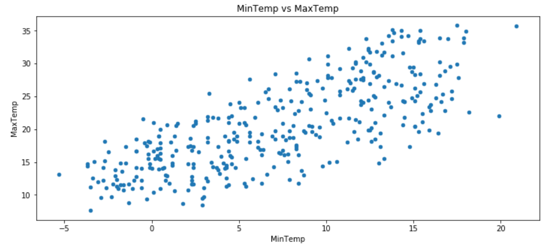

Linear regressions (LR) are pretty straightforward to do in python, but here, I want us to do it the proper way, which means splitting the data into train and test, so that we can compare performance between our LR and our neural network in a fairer manner.

线性回归(LR)在python中非常简单，但是在这里，我希望我们以正确的方式进行操作，这意味着将数据分为训练和测试，以便我们可以在LR和神经网络之间比较性能。更公平的方式。

from sklearn.model_selection import train_test_split
from sklearn.linear_model import LinearRegressionX = df.MinTemp.values.reshape(-1, 1)
y = df.MaxTemp.values.reshape(-1, 1)X_train, X_test, y_train, y_test = train_test_split(X, y, test_size=0.2)regressor = LinearRegression()  
regressor.fit(X_train, y_train)df['LR_preds'] = regressor.predict(df.MinTemp.values.reshape(-1,1))df[['MinTemp', 'MaxTemp']].plot.scatter('MinTemp', 'MaxTemp', figsize=(12,5), title="Linear Regression for MinTemp vs MaxTemp")
plt.plot(df.MinTemp, df.LR_preds, 'r');

Perfect! Now let’s see how well we do with a neural network, and for that, let’s examine the 2 fundamental parameters that can affect the results according to the theorem:

完善！ 现在，让我们看一下神经网络的性能，为此，我们根据定理研究影响结果的两个基本参数：

1. The number of neurons in our hidden layer
   隐藏层中神经元的数量
2. The activation function used in the hidden layer
   隐藏层中使用的激活功能

Let’s first examine how the number of neurons in the hidden layer can affect the approximation of the linear regression after a fixed number of training periods (also known as epochs).

让我们首先检查在固定数量的训练时间(也称为历元)后，隐藏层中神经元的数量如何影响线性回归的近似值。

from sklearn.preprocessing import MinMaxScalerscaler = MinMaxScaler()
scaler.fit(X_train)X_train = scaler.transform(X_train)
X_test = scaler.transform(X_test)from tensorflow.keras.models import Sequential
from tensorflow.keras.layers import Dense, Dropout
from tensorflow.keras.callbacks import EarlyStoppingnum_of_neurons = [1,2,3,4,5,10,20,30,50,100,500]for num_of_neuron in num_of_neurons:
     model = Sequential()     model.add(Dense(num_of_neuron))     model.add(Dense(1))     model.compile(loss='mse', optimizer='adam')     model.fit(X_train, y_train, epochs=50, validation_data=[X_test, y_test], verbose=0)     df[num_of_neuron] = model.predict(scaler.transform(df.MinTemp.values.reshape(-1, 1)))

For the same 50 epochs, you can clearly see that the more neurons you add to the hidden layer, the faster your network learns and adapts (and gets closer to the red line, our linear regression LR).

对于相同的50个时期，您可以清楚地看到，添加到隐藏层的神经元越多，网络学习和适应的速度就越快 (并接近红线，即线性回归LR)。

Adding more neurons with the same activation function to the hidden layer will merely increase the speed at which the approximation is computed.

将更多具有相同激活函数的神经元添加到隐藏层将只会提高计算近似值的速度。

Note that even if you used a single neuron and you train it for long enough, you can get to the same result as with more neurons. It just takes more time / epochs to train on.

请注意，即使您使用了单个神经元并且对其进行了足够长时间的训练，也可以获得与使用更多神经元相同的结果。 培训需要花费更多时间/时间。

Great, now let’s examine activation functions. Since we are only doing a linear regression, we should only use linear activation functions, or even no activation function since the perceptron itself works as a linear model (see below).

太好了，现在让我们研究一下激活功能。 由于我们仅进行线性回归，因此我们仅应使用线性激活函数，甚至不使用激活函数，因为感知器本身可以用作线性模型(请参见下文)。

The function within the “cell body” is the “linear” function within the perceptron. The perceptron function (wx + b) is pretty much the same as the linear function (ax + b).

“细胞体”内的功能是感知器内的“线性”功能。 感知器函数(wx + b)与线性函数(ax + b)几乎相同。

However, just out of curiosity, I did try all the keras activation functions for you guys, and below is how our linear regression would look like using a neural network compared to our original Linear Regression in red.

但是，出于好奇，我确实为你们尝试了所有的keras激活函数，下面是与我们原始的红色线性回归相比，使用神经网络的线性回归的外观。

Alright, now let’s compare the results between our Linear Regression and our Neural Network with a “linear” activation function. Note we added early stopping to avoid overfitting.

好了，现在让我们比较一下线性回归和具有“线性”激活函数的神经网络之间的结果。 请注意，我们添加了提前停止以避免过度拟合。

model = Sequential()model.add(Dense(100, activation='linear'))model.add(Dense(1))early_stop = EarlyStopping(monitor='val_loss', mode='min', patience=10)model.compile(loss='mse', optimizer='adam')model.fit(X_train, y_train, epochs=500, callbacks=[early_stop], validation_data=[X_test, y_test], verbose=0)df['NN_Final'] = model.predict(scaler.transform(df.MinTemp.values.reshape(-1, 1)))

There we have it, our linear regression model approximated by a single-layer neural network!

有了它，我们的线性回归模型可以通过单层神经网络近似！

How good is the approximation you ask? If you compare our validation MSEs (mean squared errors), they are only 0.07 apart in this example, meaning our network approximated our linear regression with a 99.6% accuracy for validation (test) MSE. Not bad at all. And I didn’t even tweak my network that much, we can certainly do better.

您要求的近似值有多好？ 如果将我们的验证MSE(均方误差)进行比较，则在本示例中它们仅相距0.07，这意味着我们的网络对线性回归进行了近似(验证(测试)MSE的准确性为99.6％ )。 一点也不差。 而且我什至没有调整我的网络，我们当然可以做得更好。

逼近多项式函数 (Approximating a Polynomial Function)

Now let’s try something a bit harder, where we actually need a proper non-linear activation function. For this proof, I will be using the famous Boston Housing Dataset available here. Let’s look at the relationship between Median House Value (our target variable) and the “% lower income” variable.

现在让我们尝试一些更困难的事情，实际上我们需要一个适当的非线性激活函数。 为了证明这一点，我将使用此处提供的著名的波士顿房屋数据集。 让我们看一下房屋中值(我们的目标变量)和“低收入百分比”变量之间的关系。

from sklearn.datasets import load_boston
boston = load_boston()df = pd.DataFrame(boston['data'], columns=['Crime Rate', 'Residential Land Zones', 'Non-retail Business Acres',
                                          'Charles River tract bounds', 'N.O. Concentration', '# of Rooms', 'Age',
                                          'Distance to Employment', 'Highway Accessibility', 'Property Tax Rate',
                                          'Pupil Teacher Ratio', 'B', '% Lower Income'])df['Median Home Value'] = boston['target'] * 10000
df = df[['% Lower Income', 'Median Home Value']]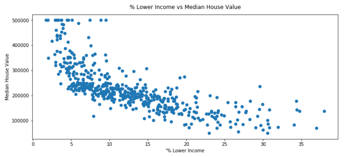

Let’s create our polynomial function and fit it to our data, using the proper way with train/test/split. Note that I am only using a polynomial of degree 2 - I tried using 3 and 4, and the MSE got worse.

让我们使用训练/测试/分割的正确方法创建多项式函数并将其拟合到数据中。 请注意，我仅使用2阶多项式-我尝试使用3和4，MSE变差了。

X = df['% Lower Income'].values.reshape(-1, 1)
y = df['Median Home Value'].values.reshape(-1, 1)X_train, X_test, y_train, y_test = train_test_split(X, y, test_size=0.2)poly = PolynomialFeatures(degree=2)X_ = poly.fit_transform(X)
X_test_ = poly.fit_transform(X_test)# Instantiate
lg = LinearRegression()# Fit
lg.fit(X_, y)# Obtain coefficients
lg.coef_arr = np.arange(0, 41, 1).reshape(-1, 1)
arr = poly.fit_transform(arr)
preds = lg.predict(arr)

Let’s create our neural network to approximate the above. This one is a bit tricky, because we have to pick a non-linear activation function to fit the data. Which one though? We will simply do an exhaustive search using all keras activation functions. Here are the results:

让我们创建我们的神经网络以近似上述。 这有点棘手，因为我们必须选择一个非线性激活函数来拟合数据。 哪一个呢？ 我们将使用所有keras激活功能简单地进行详尽搜索。 结果如下：

Looks like the exponential activation function is best, according to our validation MSE. Let’s create a full-blown neural network and compare performances between both, as we did earlier.

根据我们的验证MSE，指数激活函数似乎是最好的。 让我们创建一个成熟的神经网络，并像之前一样比较两者之间的性能。

As you can see above, by using the exponential activation function, we are able to approximate the polynomial function to a ~98.2% validation MSE similarity. Not bad at all again, and we can certainly do more tweaking if you care to go >99%. Moreover, some might argue that using an exponential function makes more sense given that as % Lower Income increases, median home value decreases.

如上所示，通过使用指数激活函数，我们能够将多项式函数近似化为约98.2％的验证MSE相似度。 一点也不差，如果您希望> 99％，我们当然可以做更多的调整。 此外，有些人可能会认为使用指数函数更有意义，因为随着低收入百分比的增加，房屋中值会下降。

结论 (Conclusion)

I hope you enjoyed reading this article as much as I enjoyed writing it! I teach data science on the side at www.thepythonacademy.com, so if you’d like further training, or even want to learn it all from scratch, feel free to contact us on the website. I also plan to publish many articles on Machine Learning and AI on here, so feel free to follow me as well. Please share, like, connect, and comment, as I always love hearing from you. Thank you!

希望您喜欢阅读这篇文章，也喜欢阅读它！ 我在www.thepythonacademy.com上提供数据科学方面的知识，因此，如果您想进行进一步的培训，或者甚至想从头开始学习，请随时与我们联系。 我还计划在此处发布有关机器学习和AI的许多文章，也可以随时关注我。 请分享，点赞，联系和评论，因为我一直很乐意收到您的来信。 谢谢！

翻译自: https://medium.com/ai-in-plain-english/universal-approximation-theorem-proof-with-code-778ac30c341b

通用逼近定理证明