


Continuing from the previous article, this one is going to approach Linear & Logistic Regression with Tensorflow and shade some light in the core differences between versions 1 and 2. Before we begin, it would be nice to discuss a little about the framework.
在上一篇文章的基础上,本篇文章将使用Tensorflow进行线性和逻辑回归 ,并为版本1和版本2之间的核心差异提供一些帮助。在开始之前,我们将对框架进行一些讨论是很不错的。
Tensorflow was originated from researchers in Google as an open source software library for Machine Intelligence for production and research. Nowadays, in its more mature version is referred as an End-to-End open source ML platform. Tensorflow, is based on graph based computation, a concept to represent mathematical calculations. Until v2, was really hard to digest and make your way out of numerous sub-apis due to lack of documentation and out-of-the-box tutorials — still. Alternatively, other frameworks such the popular Keras, came to the rescue as a wrapper library and offered a level (maybe more) layer(s) of abstraction over Tensorflow, and finally became the default in TF v2.
Tensorflow起源于Google的研究人员,它是机器智能用于生产和研究的开源软件库。 如今,在其更成熟的版本中,它被称为“ 端到端开源ML平台”。 Tensorflow基于基于图形的计算,该概念表示数学计算。 直到v2为止,由于缺乏文档和开箱即用的教程-仍然很难消化和摆脱众多子API。 或者,其他框架,如流行的Keras,作为包装库抢救过来,并在Tensorflow上提供了一个(多个)抽象层,并最终成为TF v2中的默认层。

线性回归v1 (Linear Regression v1)
Now that we are already familiar with the notion of linear regression, we can take it to a step further and train a very simple model on the linear relation between X and Y.
既然我们已经熟悉了线性回归的概念,我们可以将其进一步发展,并针对X和Y之间的线性关系训练一个非常简单的模型。
The dataset of our case study is the Birth Rate-Life expectancy. It is consists of birth rate (X) and the corresponded life expectancy (Y) for a number of countries. Assuming that the relation between them is linear Y = w*X + b we can train a model that calculates W and b.
我们的案例研究的数据集是出生率-预期寿命。 它由许多国家的出生率( X)和相应的预期寿命( Y )组成。 假设它们之间的关系为线性Y = w*X + b我们可以训练一个计算W和b的模型。
TF v1 enables us to implement the computational graph from scratch using placeholders to represent our dataset, and scalar variables for weight and bias which will be calculated with backpropagation.
TF v1使我们能够使用占位符从头开始实现计算图,以表示我们的数据集,权重和偏差的标量变量将通过反向传播进行计算。

Next we define the prediction formula with tensorflow computations and use its built-in functions for the MSE loss function and the gradient descent optimizer.
接下来,我们使用张量流计算定义预测公式,并将其内置函数用于MSE损失函数和梯度下降优化器。

Now that we have defined the components of the computational graph we need to let tensorflow know that we are going to infer our data and train the variables. This, in tf v1, is accomplished with a Session where after the graph initialisation, we infer the dataset over the computational graph. Dataset preparations techniques can be a stand alone chapter but is already simplified in v2. In this case the feed dict api is used.
现在我们已经定义了计算图的组件,我们需要让张量流知道我们将要推断数据并训练变量。 在tf v1中,这是通过一个Session完成的,其中在图形初始化之后,我们推断出计算图形上的数据集。 数据集准备技术可以是一章,但在v2中已经简化。 在这种情况下, 提要dict API 用来。

Epoch 10: | Loss: 375.46, w: 3.51, b: 41.13
Epoch 20: | Loss: 130.94, w: -0.88, b: 61.19
Epoch 30: | Loss: 59.20, w: -3.26, b: 72.10
Epoch 40: | Loss: 38.30, w: -4.56, b: 78.04
Epoch 50: | Loss: 32.29, w: -5.27, b: 81.27
Train Time: 6.204496 seconds
You may also noticed that there is a FileWriter object instantiated before the training, and that indicates a record of the computational graph visualised with Tensorboard.
您可能还会注意到,在训练之前已实例化了FileWriter对象,该对象指示使用Tensorboard可视化的计算图的记录。

By default in v1, you are not allowed to view the content of variables outside of a session and that is an issue when you have to debug your model. The only way to do that, is to enable eager execution but it does not act as a magic wand as you have to refactor you program. In latest Tensorflow’s version, eager execution is the standard default and evaluates operations immediately, without building computational graphs and thus makes it much easier to start with, as it offers a more natural flow of programming in contrast to the cumbersome style of programming in v1.
在v1中,默认情况下,不允许您在会话外部查看变量的内容,这在您必须调试模型时会遇到问题。 做到这一点的唯一方法是启用急切的执行功能,但是它不能像魔杖那样用于重构程序。 在最新的Tensorflow版本中,急切执行是标准默认设置,无需构建计算图即可立即评估操作,因此更容易上手,因为与v1中繁琐的编程风格相比,它提供了更自然的编程流程。
线性回归v2 (Linear Regression v2)
Reimplementing the linear regression model with a simple neural network in Tensorflow v2 makes it much easier to monitor computations and calculate the gradients. Let’s naively say that the new API from Keras tf.GradientTape replaced the functionality of tf.Session. GradientTape returns a Tensor object that takes over any assigned operation/calculation and can be converted to np.array too.
在Tensorflow v2中使用简单的神经网络重新实现线性回归模型,使监视计算和计算梯度变得更加容易。 让我们天真地说,从Keras新的API tf.GradientTape替代的功能tf.Session 。 GradientTape返回一个Tensor对象,该对象将接管任何分配的操作/计算,并且也可以转换为np.array 。
Weights and bias are now tf.Variable objects, something by the way in Tensorflow v1 was considered the old way of assigning variables in respect to tf.get_variable.
权重和偏差现在是tf.Variable对象,在Tensorflow v1中被认为是针对tf.get_variable.分配变量的旧方法 tf.get_variable.
Prediction, Loss function and Optimizer can now defined as simple as you write a line of code in Python
现在,您可以使用Python编写一行代码来简单地定义预测,损失函数和优化器

Training process is easier to digest and comprehend and takes less to converge than feed_dict API does.
与feed_dict API相比,培训过程更易于理解和理解,并且收敛时间更少。

Epoch: 100 | Loss: 652.59, w: 10.31, b: 30.24
Epoch: 200 | Loss: 324.81, w: 5.31, b: 47.55
Epoch: 300 | Loss: 169.67, w: 1.87, b: 59.46
Epoch: 400 | Loss: 96.24, w: -0.50, b: 67.65
Epoch: 500 | Loss: 61.48, w: -2.13, b: 73.29
Epoch: 600 | Loss: 45.03, w: -3.25, b: 77.16
Epoch: 700 | Loss: 37.24, w: -4.02, b: 79.83
Epoch: 800 | Loss: 33.56, w: -4.55, b: 81.67
Epoch: 900 | Loss: 31.81, w: -4.91, b: 82.93
Epoch: 1000 | Loss: 30.99, w: -5.17, b: 83.80
Train Time: 2.776154 seconds
逻辑回归 (Logistic Regression)
Moving forward to a more advanced implementation of Logistic Regression with a single neuron neural network, we will approach a multi-class classification problem using MNIST dataset, a collection of hand-written digits from 0 to 9.
前进到使用单个神经元神经网络的Logistic回归的更高级实现,我们将解决多类分类问题 使用MNIST数据集,从0到9的手写数字的集合。
数据准备 (Dataset preparation)
This example can be also considered a Tensorflow v1 tutorial which makes use of special terminology, built-in routines and tf.data API, a faster method comparing to placeholders and feed_dict to load a dataset.
该示例也可以被视为Tensorflow v1教程,该教程利用了特殊的术语,内置的例程和tf.data API,与占位符和feed_dict相比,它是一种更快的方法来加载数据集。

In the next step we must define a process to iterate through samples/digits of the dataset, let’s say an iterator. Each time a new batch/sample is being processed is called the get_next(). Constructing the classifier, we will not process the data samples one by one as this will slow down the training due to the dataset size. Thus we are going to process the data in batches to accelerate the process. We also explicitly define not to discard the remaining samples in the last batch when iterating(train & test), if it does not fit in the training set with drop_remainder=False
在下一步中,我们必须定义一个过程来迭代数据集的样本/数字,比如说iterator 。 每次处理新的批次/样品都称为get_next() 。 构造分类器时,我们不会一一处理数据样本,因为由于数据集的大小,这会减慢训练速度。 因此,我们将分批处理数据以加快流程。 我们还明确定义了在迭代(train&test)时不丢弃最后一批中的剩余样本(如果它不适合drop_remainder=False的训练集)
After every epoch, tensorflow needs to rewind the dataset and continue to the next epochs. The initialisation operation is defined with a iterator.make_initializer()object, fed with the part of the dataset.
在每个时期之后,张量流需要倒退数据集并继续到下一个时期。 初始化操作是通过iterator.make_initializer()对象定义的,该对象与数据集的一部分一起提供。
We will elaborate more about how the batches consumed in the training process in a next section.
在下一部分中,我们将详细说明培训过程中批次的消耗方式。

In this case, weights and bias have to follow the dimensions of the dataset as well.
在这种情况下,权重和偏差也必须遵循数据集的维度。

计算损失 (Calculate Loss)
Tensorflow uses the term logits or unscaled log probabilities, which actually is the output of the model during forward propagation before any other operation is applied.
Tensorflow使用术语logits或未缩放的对数概率 ,这实际上是模型在进行任何其他操作之前的正向传播过程中的输出。
How much of these probabilities lead to correct prediction is measured with cross-entropy which a) applies a softmax activation on logits, converting the output to normalised probabilities summed to 1 aka predictions and b) computes the distance from the ground truth.
使用交叉熵来衡量这些概率中有多少导致正确的预测 其中a)在logit上应用softmax激活 ,将输出转换为归纳为1 aka 预测的归一化概率,并且b)计算与地面真相的距离。

The total loss is calculated from the mean value of the total training instances.
根据总训练实例的平均值计算总损失。

# Sample output from a single 128 size batch# Logits (10,128)
[[-0.02467263  0.0407119   0.03357347 ...  0.07849845 -0.04018284
   0.14606732]
...
[-0.03187682  0.03064402  0.02814235 ...  0.12632789 -0.07327773
   0.16343306]]# Softmax + Cross Entropy (128,)
[2.280719  2.3213248 ... 2.2659633 2.3112588]# Batch Loss
2.315973
优化器 (Optimizer)
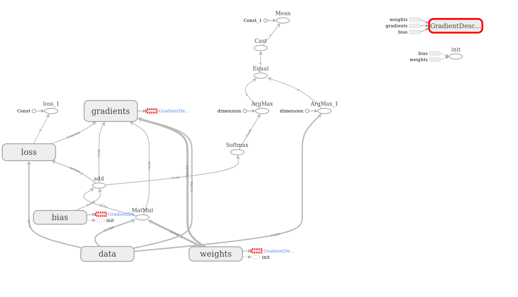
In tensorflow’s dialect, optimizer is an operation and is used to minimise loss. It is executed in a session.run(), passed in a list along with loss computation. This is because, the calculation graph of Tensorflow executes the parts that optimizer is depended such loss and loss depends on input data and weights and bias as well. That can be seen from the following graph, produced in tensorboard.
在tensorflow的方言中,优化器是一种操作 ,用于最大程度地减少损失。 它在session.run()执行,并与损失计算一起传递到列表中。 这是因为,Tensorflow的计算图执行了优化器所依赖的部分,这种损失和损失也取决于输入数据,权重和偏差。 这可以从张量板上生成的下图看出。
optimizer=tf.train.GradientDescentOptimizer(0.001).minimize(loss)# Training process
_, batch_loss, batch_acc = sess.run([optimizer, loss, accuracy])
准确性和混淆矩阵 (Accuracy & Confusion Matrix)
Model’s performance is not only assessed with loss, but also with the a range of statistical metrics. In this example, model is evaluated in accuracy of the classifier to produce correct predictions along with a confusion matrix (precision, recall) with actual vs predicted class.
模型的性能不仅可以通过损失来评估,还可以通过一系列统计指标来评估。 在此示例中,对模型进行分类器的准确性评估,以产生正确的预测以及带有实际与预测类的混淆矩阵(精度,召回率) 。

# Sample output from a single 128 size batch# Predictions (10,128)
[[0.099 0.10 0.11 ... 0.08 0.09 0.09]
...
[0.11 0.10 0.09  ... 0.08 0.10 0.10]]# Correct Preds (128,)
[False True ... False False]# Batch Accuracy
0.078------------------------------------------------------------------Training...
Epoch 10 - Train loss: 0.875 - Train Accuracy: 83.16%
Epoch 20 - Train loss: 0.653 - Train Accuracy: 85.49%
Epoch 30 - Train loss: 0.564 - Train Accuracy: 86.53%
Epoch 40 - Train loss: 0.515 - Train Accuracy: 87.21%
Epoch 50 - Train loss: 0.483 - Train Accuracy: 87.73%
Epoch 60 - Train loss: 0.460 - Train Accuracy: 88.10%
Evaluating...
Test Validation loss: 0.067, Validation Accuracy: 89.09%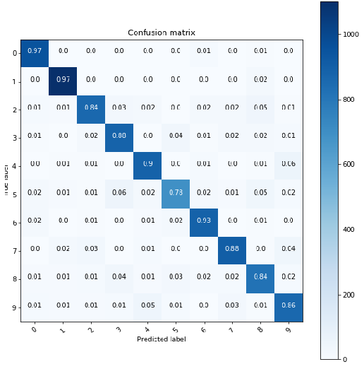
培训和批处理 (Training and batch processing)
Feeding the computational graph with data from an iterator is a process that has to be implemented in a semi-manual way. In every epoch, the iterator handles the dataset per batch size and for each batch loss, accuracy and batch cycles, are computed in order to calculate the total loss and accuracy for each epoch.
向计算图提供来自迭代器的数据是必须以半手动方式实现的过程。 在每一个时期中,迭代处理每批量大小和每批损失 ,准确性和批次周期数据集,以便计算用于每个历元的总损耗和精度计算。

For example in a train dataset of 55K samples and batch_size=128the batch_cyclewill be 430 times, when drop_remainder=Falseand 429 when is True.
例如在55K样本和列车数据集batch_size=128的batch_cycle将430倍,当drop_remainder=False是当和429 True 。
The latter means that when an epoch needs one more batch to complete, it just discards it and depletes the iterator immediately at (128x429=54912 samples)
后者意味着当一个纪元需要再完成一个批处理时,它将被丢弃并立即消耗迭代器( 128x429 = 54912个样本 )
结论 (Conclusions)
This article completes an extended explorations in regression. If you are a beginner and haven’t invested much time to deepen on how a computational graph works and does all the magic under the hood, tensorflow version 1.x gives you the chance!
本文完成了回归的扩展探索。 如果您是新手,并且没有花太多时间来深入了解计算图的工作原理以及如何在幕后进行所有操作,tensorflow 1.x版将为您提供机会!
In a next article we will make a multilayer perceptron (MLP) learn the Tensorflow’s playground datasets.
在下一篇文章中,我们将使多层感知器(MLP)学习Tensorflow的游乐场数据集。
Source code: https://github.com/sniafas/ML-Projects/tree/master/Regression
源代码: https : //github.com/sniafas/ML-Projects/tree/master/Regression
[2] https://www.tensorflow.org/guide/autodiff
[2] https://www.tensorflow.org/guide/autodiff
[3] https://www.easy-tensorflow.com/tf-tutorials/basics/introduction-to-tensorboard
[3] https://www.easy-tensorflow.com/tf-tutorials/basics/introduction-to-tensorboard
翻译自: https://medium.com/@sniafas/regression-in-tensorflow-v1-v2-e8d7e80068b


 701
701

 被折叠的 条评论
为什么被折叠?
被折叠的 条评论
为什么被折叠?
 到【灌水乐园】发言


