机器人影视对接_机器学习对接会

机器人影视对接

A simple question like ‘How do you find a compatible partner?’ is what pushed me to try to do this project in order to find a compatible partner for any person in a population, and the motive behind this blog post is to explain my approach towards this problem in a manner as clear as possible.

一个简单的问题，例如“如何找到兼容的合作伙伴？” 是促使我尝试执行此项目的原因，以便为人群中的任何人找到兼容的合作伙伴，而本博客文章的动机是，以尽可能清晰的方式解释我对这一问题的解决方法。

You can find the project notebook here.

您可以在 此处 找到项目笔记本 。

If I asked you to find a partner, what would be your next step? And what if I had asked you to find a compatible partner? Would that change things?

如果我要您找到合作伙伴，下一步将是什么？ 如果我要您找到兼容的合作伙伴怎么办？ 这会改变一切吗？

A simple word such as compatible can make things tough, because apparently humans are complex.

诸如兼容之类的简单词会使事情变得艰难，因为显然人类是复杂的。

数据 (The Data)

Since we couldn’t find any single dataset that could cover the variation in persona, we resorted to using the Big5 personality dataset, Interests dataset (also known as Young-People-Survey dataset) and Baby-Names dataset.

由于找不到任何可以覆盖角色差异的数据集，因此我们诉诸使用Big5人格数据集 ， 兴趣数据集 (也称为Young-People-Survey数据集)和Baby-Names数据集 。

Big5 personality dataset: The reason we are choosing Big5 dataset is solely because it provides an idea about any individual’s personality through the Big5/OCEAN personality test which asks a respondent 50 questions, 10 questions each for Openness, Conscientiousness, Extraversion, Agreeableness & Neuroticism to measure them on a scale of 1–5. You can read more about Big5 here.

Big5人格数据集 ：我们之所以选择Big5数据集，完全是因为它通过Big5 / OCEAN人格测验提供了有关任何人的性格观念，该测验向被访者询问50个问题，每个问题中有10个问题涉及开放性，尽责性，性格外向，愉快和神经质。用1–5的比例尺测量它们。 您可以在此处阅读有关Big5的更多信息。

Interests dataset: which covers the interests & hobbies of a person by asking them to rate 50 different areas of interest (such as art, reading, politics, sports etc.) on a scale of 1-5.

兴趣数据集：涵盖一个人的兴趣和爱好 ，要求他们以1-5的等级对50个不同的兴趣领域(例如艺术，阅读，政治，体育等)进行评分。

Baby-Names dataset: helps in assigning a real and unique name to each respondent

婴儿名字数据集：有助于为每个受访者分配真实唯一的名字

The project is made in R language (version 4.0.0)With the help of dplyr and cluster packages

在dplyr和集群软件包的帮助下，该项目以R语言(版本4.0.0)完成

处理中 (Processing)

Loading the Big5 dataset, which has 19k+ observations with 57 variables including Race, Age, Gender, Country besides the personality questions.

正在加载Big5数据集，该数据集具有19k +个观察值，其中包括57个变量，包括种族，年龄，性别，国家/地区以及人格问题。

Removing the respondents who did not respond to few questions & some respondents with vague age values such as: 412434, 223, 999999999

删除没有回答几个问题的受访者和年龄值不明确的一些受访者，例如：412434、223、99999999

Taking a healthy sample of 5000 respondents, since we don’t want the laptop go for a vacation when we want to find Euclidean distances between thousands of observations for clustering :)

对5000名受访者进行了健康的抽样调查，因为当我们想要找到成千上万个观测值之间的欧几里得距离进行聚类时，我们不想让笔记本电脑去度假：)

Loading the Baby-Names dataset and adding 5000 unique and real names to identify each observation as a person than just a number.

加载Baby-Names数据集并添加5000个唯一和真实的名称，以将每个观察值识别为一个人而不是一个数字。

Loading the Interests dataset, the dataset has 50 variables, each of them an interest or a hobby

加载兴趣数据集后，该数据集包含50个变量，每个变量都是兴趣或嗜好

The heatmap shows us that some areas such as medicine, chemistry; theatre, musical; and politics, history show some correlation. This observation is important, as we will be using this knowledge ahead.

该热图向我们展示了某些领域，例如医学，化学； 剧院，音乐剧； 与政治，历史显示出一定的关联。 此观察很重要，因为我们将在前面使用这些知识。

After loading all of the datasets we combine them into one master dataframe and name it train, which has 107 column which are shown here:

加载所有数据集后，我们将它们组合到一个主数据框中并命名为train，该列具有107列，如下所示：

A few plots to see how our data lays out in terms of Age and Gender

一些图表可以看出我们的数据在年龄和性别方面的布局

We can see majority of respondents is youth, and we have more female respondents than male

我们可以看到大多数受访者是青年，女性受访者比男性多

主成分分析 (Principal Component Analysis)

Remember we saw little correlation in the heatmap? Well this is where the Principal Component Analysis comes in. PCA combines the effect of some similar columns into a Principal Component column or PC.

还记得我们在热图中没有看到多少相关性吗？ 好的，这就是进行主成分分析的地方。PCA将一些类似的列的效果合并到了“主成分”列或PC中。

For those who don’t know what Principal Component Analysis is; PCA is a dimension reduction technique which focuses on creating a totally new variable or a Principal Component(PC for short) from all of the variables through an equation to grasp most variation possible, from the data.

对于那些不知道什么是主成分分析的人； PCA是一种降维技术，其重点是通过方程式从所有变量中创建一个全新的变量或主成分(简称PC)，以从数据中把握最大的变化。

In simple terms, PCA will help us in using only a few components which take into account the most important and most varying variables instead of using all 50 variables. You can learn more about PCA here.

简而言之，PCA将帮助我们仅使用几个考虑了最重要且变化最大的变量的组件，而不是全部使用50个变量。 您可以在此处了解有关PCA的更多信息。

Important: We run PCA on Interests columns and Big5 columns separately, since we don’t want to mix interests & personality.

重要提示 ：由于我们不想混合兴趣和个性，因此我们分别在兴趣列和Big5列上运行PCA。

After running the PCA on Interest columns, what we get is 50 PCs. Now here is the fun part, we won’t be using all of them, here’s why: the first PC would be the strongest i.e a column that will grasp most of the variation in our data, the second PC would be weaker, and will grasp lesser variation and so on until 50th PC.

在“兴趣”列上运行PCA之后，我们得到的是50台PC。 现在这是有趣的部分， 我们不会使用所有这些 ，这是为什么：第一台PC将是最强大的，即一列将掌握我们数据的大部分变化，第二台PC将更弱，并且将掌握较小的变化，依此类推，直到第50台PC。

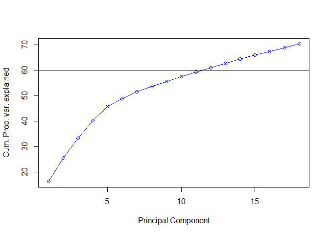
Our objective is to find the sweet spot between using 0 and 50 PCs and we will do that by plotting the variance explained by the PCs:

我们的目标是找到使用0到50台PC之间的最佳点，我们将通过绘制PC解释的方差来做到这一点：

The plots show us the Proportion of Variation explained by each PC. Left: Each PC’s individual performance is shown (for example, the first PC explains around 10% of the variation in our data, but the 15th one only 2%)
Right: Cumulative version of the plot on the left.

这些图向我们展示了每台PC解释的变化比例。 左：显示了每台PC的个人性能(例如，第一台PC解释了我们数据变化的大约10％，而第15台仅解释了2％) 右：左侧图的累积版本。

We see that after 10 PCs there is very low individual contribution.
But we will stretch it a little bit to cover 60% variance & take out 14 PCs.

我们看到10台PC之后，个人贡献非常低。 但是我们将稍微扩展一下以涵盖60％的差异并取出14台PC。

The result? we just shrank number of columns from 50 to just 14, which explain 60% of the variation in the original Interest columns.

结果？ 我们只是将列数从50缩减为14 ，这可以解释原始兴趣列的变化的60％。

Similarly, we do PCA on Big5 columns:

同样，我们在Big5列上执行PCA：

Again we see the first PC is the strongest, and explains more than 16% of the variance. 再次，我们看到第一台PC最强，并解释了超过16％的方差。

While the slope starts flattening after 8th PC, we will go with 12, to grasp around 60% of the variance. 当斜率在第8个PC之后开始变平时，我们将使用12，以掌握大约60％的方差。

Now that we have reduced the columns in Big5 from 50 to 14 , and in Interests from 50 to 12, we combine them into a dataframe different from train. We call it pcatrain.

现在，我们已将Big5中的列从50减少到14 ，将Interests从50减少到12 ，我们将它们组合成不同于train的数据帧。 我们称它为pcatrain。

A glimpse of the pcatrain dataframe with the column names

列名对pcatrain数据框的了解

聚类 (Clustering)

As a good practice we first use Hierarchical Clustering to find a good value for k (the number of clusters)

作为一种好的做法，我们首先使用层次聚类为k (聚类数)找到一个好的值

层次聚类 (Hierarchical Clustering)

What is Hierarchical Clustering? Here is an example: Think of a house party of 100 people, now we start with every single person representing as a cluster of 1 person. The next step? We combine the two people/clusters standing closest into one cluster, then we label another two closest clusters as one, and so on. Finally we have gone from 100 clusters to 1 cluster. What Hierarchical Clustering does is form clusters on the basis of distance between the clusters and then we can see that process in a dendogram.

什么是层次聚类？ 这是一个示例：假设有一个100人的家庭聚会，现在我们从每个人代表一个1人的集群开始。 下一步？ 我们将最靠近的两个人/集群合并为一个集群，然后将另外两个最近的集群标记为一个，依此类推。 最终，我们从100个群集变为1个群集。 层次聚类所做的是基于聚类之间的距离形成聚类，然后我们可以在树状图中看到该过程。

The red line might be a cutoff point

红线可能是截止点

After doing Hierarchical Clustering we can see our own cluster dendogram here, as we go from bottom to top we see every cluster converging, the more distant each cluster is from the other, the longer steps it takes to converge; which you can see by looking at the vertical joins.

完成分层聚类后，我们可以在此处看到自己的聚类树状图，当我们从下往上看时，每个聚类都在收敛，每个聚类之间的距离越远，收敛所需的时间就越长； 您可以通过查看垂直联接来看到。

Based on the distance we use the red line to divide a healthy group of 7 diverse clusters. The reason behind 7 is that, the 7 clusters take longer steps to converge, i.e the clusters are distant.

根据距离，我们使用红线将健康的组划分为7个不同的簇。 7背后的原因是，这7个聚类需要更长的时间才能收敛，即聚类较远。

K均值聚类 (K-Means Clustering)

We use Elbow Method in K-Means to make sure that taking around 7 clusters is a good choice, we wont dive deep into it, but to summarize: The marginal sum of within-cluster distances between individuals & the marginal distance between the cluster centers is best at 6 clusters.

我们 在K-Means中 使用 Elbow方法 来确保大约7个聚类是一个不错的选择，我们不会深入研究它，而是总结一下：个人之间的聚类内距离的边际总和以及聚类中心之间的边际距离 最好 是 在6簇 。

具有6个聚类的K-Means聚类 (K-Means clustering with 6 clusters)

We run K-Means clustering with k=6; check the size of each cluster; what cluster the first 10 people are assigned. Finally we add this cluster column to our pcatrain dataframe, and now our dataframe has 33 columns.

我们以k = 6进行K-Means聚类； 检查每个群集的大小； 前十个人被分配到哪个集群。 最后，我们将此簇列添加到我们的pcatrain数据帧中，现在我们的数据帧具有33列。

最后步骤 (Final steps)

Now that we have assigned clusters, we can start finding close matches for any individual.

现在，我们已经分配了集群，我们可以开始查找任何个体的紧密匹配项。

We select Penni as a random individual, for whom we will find matches from her cluster i.e cluster 2

我们选择Penni作为随机个体，我们将从其簇中找到匹配，即簇2

On left, we first find people from Penni’s cluster, then filter out people those who are in the same country as Penni’s, opposite gender, and belong to Penni’s age category.

在左侧，我们首先从Penni的族群中找到人，然后过滤掉与Penni处于同一国家，性别相反并且属于Penni的年龄类别的人。

Some people who belong to same cluster, country, age-group as Penni’s

与Penni属于同一族群，国家，年龄组的人

Okay so now we have filtered out people, is that it?

好吧，现在我们已经滤除人员了，是吗？

No. Remember the question we asked in the beginning?

否。还记得我们一开始提出的问题吗？

‘How do you find a compatible partner?’

“您如何找到兼容的合作伙伴？”

Even though we have found people with same interests and age-group, we must find people who have personality most similar to Penni’s.

即使我们发现了具有相同兴趣和年龄段的人 ， 我们也必须找到与Penni的人格最相似的人。

This is where the Big5 personality columns come in handy.

这是Big5个性专栏派上用场的地方。

Through Big5, we will be able to find people who have the same level of Openness, Conscientiousness, Extraversion, Agreeableness and Neuroticism as Penni’s.

通过Big5，我们将能够找到与Penni's具有相同程度的开放性，尽责性，性格外向，和gree可亲和神经质的人。

What we did here is find the difference between the response of Penni and the response of filtered people for each personality column, and then added the differences of all the columns .

我们在这里所做的是找到每个个性列的Penni响应与被过滤人员的响应之间的差异 ，然后加上所有列的差异。

For example: Brody has sumdifference = 8.9, i.e In 50 questions of Big5, Brody’s responses differ by only 8.9 points from Penni’s responses. 例如：Brody的总和= 8.9，即在Big5的50个问题中，Brody的回答与Penni的回答仅相差8.9分。

So now we know, if Penni is looking for a partner, she should first try to meet Brody.

因此，现在我们知道，如果Penni正在寻找伴侣，她应该首先尝试与Brody见面。

我们为Penni寻找兼容人所做的工作的摘要： (A summary of what we did to find a compatible person for Penni:)

1. Clustered people on the basis of their interests.
   根据他们的兴趣聚集人们。
2. Found people who have similar interests, belong to same age-group as Penni’s.
   发现兴趣相似的人，与Penni属于同一年龄段。
3. Ranked those filtered people on the basis of how closely their personality matches Penni’s personality.
   根据他们的人格与Penni的人格相匹配的程度对这些被过滤的人进行排名。

Thank you for sticking till the end!

感谢您坚持到底！

You can connect with me on:

您可以通过以下方式与我联系：

Github

Github

LinkedIn

领英

翻译自: https://towardsdatascience.com/machine-learning-matchmaking-4416579d4d5e

机器人影视对接