


web数据交互
Most good data projects start with the analyst doing something to get a feel for the data that they are dealing with.
大多数好的数据项目都是从分析师开始做一些事情,以便对他们正在处理的数据有所了解。
They might hack together a Jupyter notebook to look at data summaries, first few rows of data and matplotlib charts. Some might look through the data as an Excel sheet and fidget with pivot tables. The ones truly one with the data might even prefer to stare directly at the raw table of data.
他们可能会聚在一起使用Jupyter笔记本来查看数据摘要,数据的前几行和matplotlib图表。 有些人可能会将数据视为Excel工作表和带有数据透视表的小工具。 真正拥有数据的人甚至可能更喜欢直接盯着原始数据表。
None of these are ideal solutions. Some of these solutions might be only suitable for the masochistic among us. So what is a person to do?
这些都不是理想的解决方案。 其中一些解决方案可能仅适用于我们中间的受虐狂。 那么一个人该怎么办?
For me, I prefer to build a web app for data exploration.
对我来说,我更喜欢构建一个用于数据探索的Web应用程序。
There’s something about the ability to slice, group, filter, and most importantly — see the data, that helps me to understand it and help me to formulate questions and hypotheses that I want answered in the .
关于切片,分组,过滤的功能,最重要的是- 查看数据,这有助于我理解数据,并帮助我提出要在回答的问题和假设。
It allows me to interact with the data visually.
它使我可以直观地与数据进行交互 。
My preferred toolkit of choice for this task these days is Plotly and Streamlit. I’ve written enough about Plotly over the last while — I think it’s the best data visualisation package out there for Python. But Streamlit has really changed the way I work. Because it is so terse, it takes almost no extra effort to turn my plots and comments in a python script into a web app with interactivity as I tinker. (FYI — I wrote a comparison between Dash and Streamlit here)
这些天,我首选的首选工具包是Plotly和Streamlit 。 上一阵子我已经写了足够多的有关Plotly的文章-我认为这是Python最好的数据可视化软件包。 但是Streamlit确实改变了我的工作方式。 因为它是如此的简洁,所以我几乎不需要花费额外的精力就可以将python脚本中的绘图和注释转换为具有交互性的Web应用程序。 (仅供参考-我在这里写了Dash和Streamlit之间的比较 )
I prefer to build a web app for data exploration
我更喜欢构建用于数据探索的Web应用程序
So in this article, I’d like to share with a simple example building a data exploration app with these tools.
因此,在本文中,我想与一个使用这些工具构建数据探索应用程序的简单示例分享。
Now, for a data project – we need data, and here I will be using stats from the NBA. Learning programming can be dry, so using something relatable like sports data helps me to stay engaged; and hopefully it will for you too.
现在,对于数据项目,我们需要数据,在这里,我将使用NBA的统计数据。 学习编程可能很枯燥,因此使用诸如体育数据之类的相关内容有助于我保持专注。 希望它也对您有用。
(Don’t worry if you don’t follow the NBA as the focus is on the data science and programming!)
(如果您不关注NBA,请不要担心,因为重点是数据科学和编程!)
在开始之前 (Before we get started)
To follow along, install a few packages — plotly, streamlit and pandas. Install each (in your virtual environment) with a simple pip install [PACKAGE_NAME].
plotly ,请安装一些软件包plotly , streamlit和pandas 。 通过简单的pip install [PACKAGE_NAME]安装每个组件(在您的虚拟环境中)。
The code for this article is on my GitHub repo here, so you can download/copy/fork away to your heart’s content.
本文的代码位于我的GitHub存储库中 ,因此您可以下载/复制/分叉到您的内心。
The script is called data_explorer_app.py — so you can run it from the shell with:
该脚本名为data_explorer_app.py ,因此您可以使用以下命令从Shell运行该脚本:
streamlit run data_explorer_app.pyOh, this is the first in a set of data science / data analysis articles that I plan to write about using NBA data. It’ll all go to that repo, so keep your eyes peeled!
哦,这是我计划就使用NBA数据撰写的一组数据科学/数据分析文章中的第一篇。 一切都会去那个仓库,所以要睁大眼睛!
If you are following along, import the key libraries with:
如果您遵循以下步骤,请使用以下命令导入密钥库:
import pandas as pd
import plotly.express as px
import streamlit as st
And we are ready to go.
我们已经准备好出发了。
数据深度潜水 (Data Deep Diving)
流式照明 (Streamlit-ing)
We use Streamlit here, as it is designed to help us build data apps quickly. So what we are going to build is a Streamlit app that will then run locally. (For more information — you can check out my Dash v Streamlit article here.)
我们在这里使用Streamlit,因为它旨在帮助我们快速构建数据应用程序。 因此,我们要构建的是Streamlit应用程序,该应用程序然后将在本地运行。 (有关更多信息,您可以在此处查看我的Dash v Streamlit文章 。)
If you’ve never used Streamlit, this is all you need to build bare-bones app:
如果您从未使用过Streamlit,这就是构建准系统应用程序所需要的:
import streamlit as st
st.write("Hello, world!")
Save this as app.py, and then execute it with a shell command streamlit run app.py:
将其另存为app.py ,然后使用shell命令streamlit run app.py执行它:

And you have a functioning web app! Building a streamlit app is that easy. Even more amazingly, though, building a useful app isn’t much harder.
而且您有一个运行良好的Web应用程序! 构建流式应用很容易。 但是,更令人惊讶的是,构建有用的应用程序并不难。
Oh, by the way, you don’t need to stop and restart the server every time the script is changed. Whenever the underlying script file is updated, you will see a button pop-up on the top right corner like so:
哦,顺便说一句,您不必在每次更改脚本时都停止并重新启动服务器。 每当基础脚本文件更新时,您都会在右上角看到一个按钮弹出,如下所示:
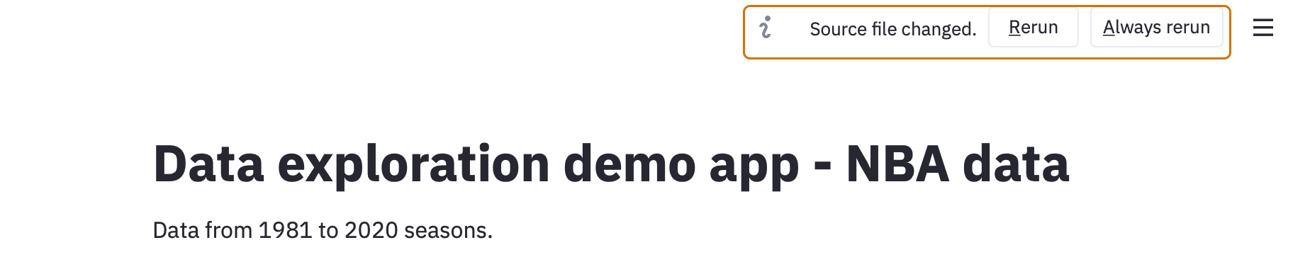
Just keep the script running, and hit Rerun here every time you want to see the latest version at work.
只需保持脚本运行,然后在每次要查看最新版本时都单击“重新运行”即可。
Ready? Okay, let’s go!
准备? 好吧,走吧!
原始数据探索 (Raw data exploration)
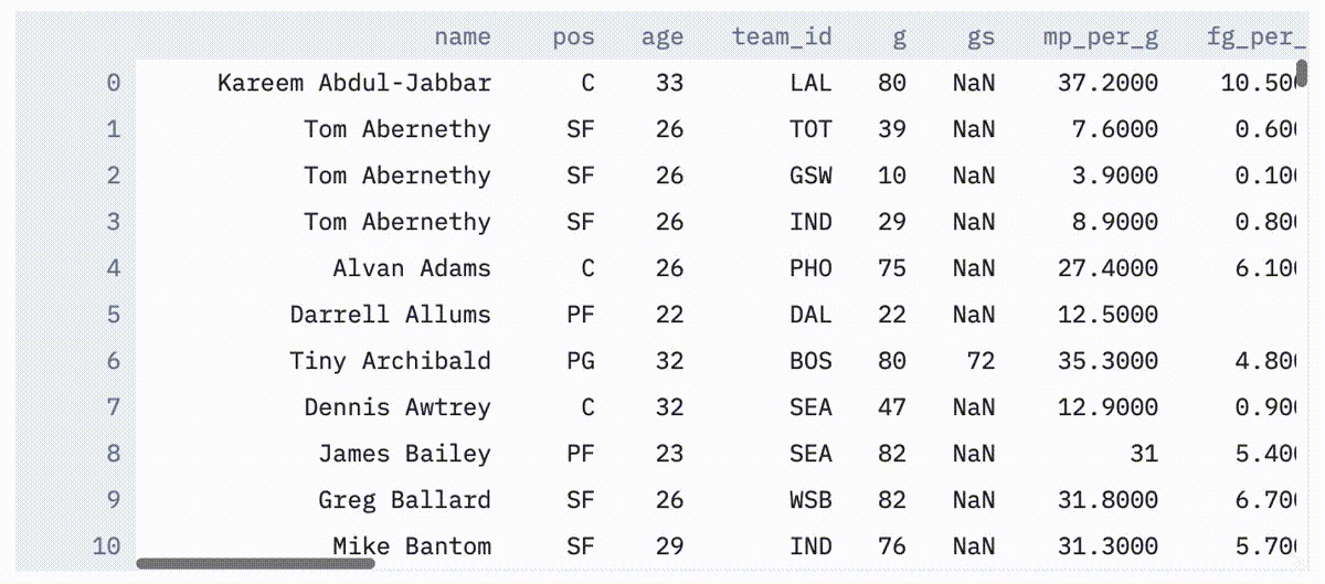
What I like to do initially it to look at the entire raw dataset. As a first step, we load the data from a CSV file:
我最初想要做的是查看整个原始数据集。 第一步,我们从CSV文件加载数据:
df = pd.read_csv("data/player_per_game.csv", index_col=0).reset_index(drop=True)Once the data has been loaded, simply typing st.write(df) creates a dynamic, interactive table of the entire dataframe.
加载数据后,只需键入st.write(df)创建整个数据帧的动态交互式表。
And the various statistics for columns can be similarly plotted with st.write(df.describe()).
并且可以使用st.write(df.describe())类似地绘制列的各种统计信息。

I know you can plot a table in Jupyter notebooks, but the difference is in the interactivity. For one, tables rendered with Streamlit are sortable by columns. And as you will see later, you can incorporate filters and other dynamic elements that aren’t as easy to incorporate in notebooks — which is where the real power comes in.
我知道您可以在Jupyter笔记本中绘制表格,但区别在于交互性。 首先,使用Streamlit渲染的表可以按列排序。 就像您稍后将看到的那样,您可以合并过滤器和其他动态元素,而这些元素和合并到笔记本中并不那么容易-这才是真正的动力所在。
Now we are ready to start adding a few charts to our app.
现在,我们准备开始向我们的应用程序添加一些图表。
分布可视化 (Distribution visualisations)
Statistical visualisation of individual variables are extremely useful, to an extent that I think it’s an indispensable tool above and beyond looking at the raw data.
单个变量的统计可视化非常有用,在某种程度上,我认为它是查看原始数据之外不可或缺的工具。
We will begin the analysis by visualising the data by one variable, with an interactive histogram. A histogram can be constructed with Plotly like so:
我们将通过交互式变量直方图通过一个变量将数据可视化来开始分析。 可以使用Plotly构造直方图,如下所示:
hist_fig = px.histogram(df, x=hist_x, nbins=hist_bins)Traditionally, we would have to manually adjust the x and nbins variables to see what happens, or create a huge wall of histograms from various permutations of these variables. Instead, let’s see how they can be taken in as inputs to interactively investigate the data.
传统上,我们将不得不手动调整x和nbins变量以查看会发生什么,或者从这些变量的各种排列中创建巨大的直方图墙。 相反,让我们看看如何将它们作为交互研究数据的输入。
The histogram will analyse data from one column of the pandas dataframe. Let’s render it as a drop-down box by calling the st.selectbox() module. We can just grab a list of the columns as df.columns, and additionally we provide a default choice, which we get the column number of using df.columns.get_loc() method. Putting it together, we get:
直方图将分析来自熊猫数据框一列的数据。 通过调用st.selectbox()模块,将其呈现为下拉框。 我们可以仅以df.columns获取列的列表,此外,我们还提供了一个默认选择,即使用df.columns.get_loc()方法获得列号。 放在一起,我们得到:
hist_x = st.selectbox("Histogram variable", options=df.columns, index=df.columns.get_loc("mp_per_g"))Then, a slider can be called with the st.slider() module for the user to select the number of bins in the histogram. The module can be customised a minimum/maximum/default and increment parameters as you see below.
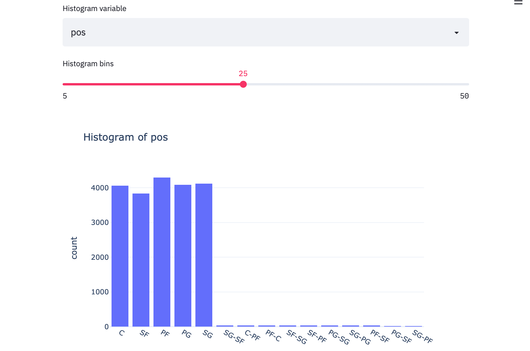
然后,可以使用st.slider()模块调用滑块,以供用户选择直方图中的bin数量。 您可以自定义模块的最小/最大/默认和增量参数,如下所示。
hist_bins = st.slider(label="Histogram bins", min_value=5, max_value=50, value=25, step=1)These parameters can then be combined to produce the figure:
然后可以将这些参数组合以产生图形:
hist_fig = px.histogram(df, x=hist_x, nbins=hist_bins, title="Histogram of " + hist_x,
                        template="plotly_white")
st.write(hist_fig)
Putting it together with a little heading st.header(“Histogram”), we get:
将其与一个小标题st.header(“Histogram”)放在一起,我们得到:
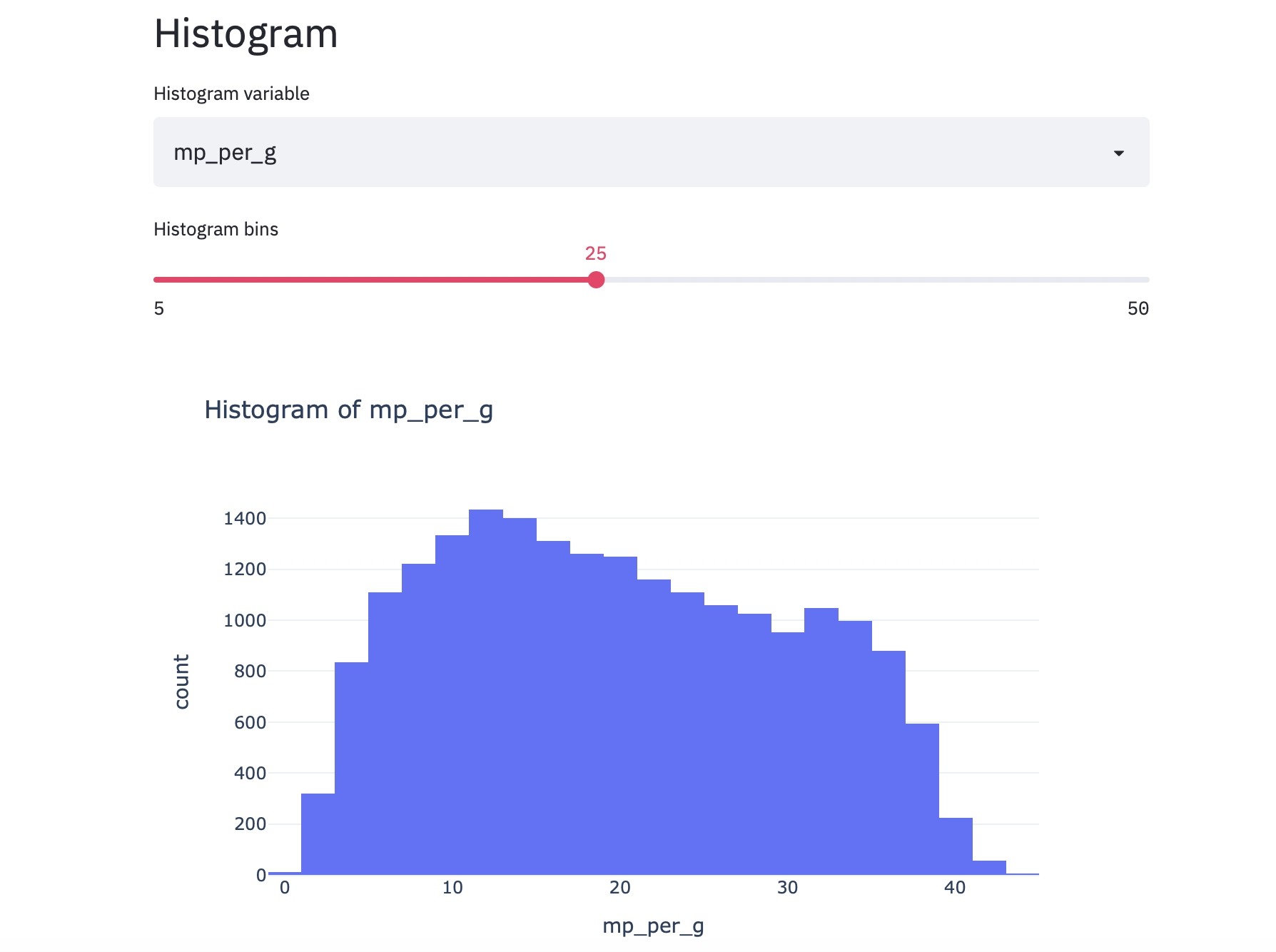
I recommend taking a second here to explore the data. For example, take a look at different stats like rebounds per game:
我建议在这里花点时间浏览数据。 例如,看一下不同的统计数据,例如每场比赛的篮板数:
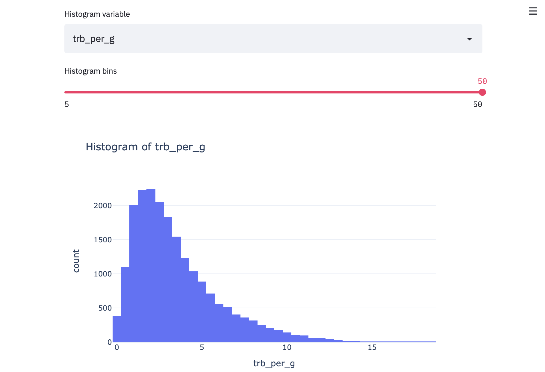
Or positions:
或职位:
The interactivity makes for easier, dynamic, active exploration of the data.
交互性使对数据的更轻松,动态, 主动的 探索成为可能。
You might have noticed in this last graph that the histogram categories are not in any sort of sensible order. This is due to the fact that this is a categorical variable. So without a provided order, Plotly is (I think) plotting these categories based on the order that it starts to encounter each category for the first time. So, let’s make one last change to would fix that.
您可能已经在最后一张图中注意到,直方图类别没有任何合理的顺序。 这是由于这是一个类别变量。 因此,如果没有提供的顺序,Plotly(我认为)将根据第一次遇到每个类别的顺序来绘制这些类别。 因此,让我们做最后一个更改来解决该问题。
Since Plotly allows for a category_orders parameter, we could pass a sorted order of positions. But then it wouldn’t be relevant for any of the other parameters. Instead, what we can do is to isolate the column based on the chosen input value, and pass them on by sorting them alphabetically like so:
由于Plotly允许有category_orders参数,因此我们可以传递排名的排序顺序。 但这与其他任何参数都不相关。 相反,我们可以做的是根据所选的输入值隔离列,然后按字母顺序对它们进行传递,如下所示:
df[hist_x].sort_values().unique()All together, we get:
总之,我们得到:
hist_cats = df[hist_x].sort_values().values
hist_fig = px.histogram(df, x=hist_x, nbins=hist_bins, title="Histogram of " + hist_x,
                        template="plotly_white", category_orders={hist_x: hist_cats})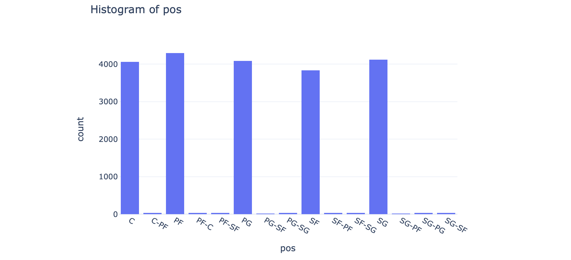
This way, any categorical (or ordinal) variables would be presented in order
这样,任何分类(或有序)变量将按顺序显示
Now we can go another step and categorise our data with boxplots. Boxplots do a similar job as histograms in that they show distributions, but they are really best at showing how those distributions changed according to another variable.
现在,我们可以再进行一步,用箱线图对数据进行分类。 箱线图的功能与直方图类似,因为它们可以显示分布,但实际上最能显示出这些分布如何根据另一个变量而变化。
So, the boxplot portion of our app is going to include two pulldown menus like below.
因此,我们应用程序的箱线图部分将包括两个下拉菜单,如下所示。
box_x = st.selectbox("Boxplot variable", options=df.columns, index=df.columns.get_loc("pts_per_g"))
box_cat = st.selectbox("Categorical variable", ["pos_simple", "age", "season"], 0)
And it’s just a matter of passing those two inputs to Plotly to build a figure:
只需将这两个输入传递给Plotly即可构建图形:
box_fig = px.box(df, x=box_cat, y=box_x, title="Box plot of " + box_x, template="plotly_white", category_orders={"pos_simple": ["PG", "SG", "SF", "PF", "C"]})
st.write(box_fig)
Then… voila! You have an interactive box plot!
然后……瞧! 您有一个交互式箱形图!

You will notice here that I manually passed an order for my simplified positions column. The reason is that this order is a relatively arbitrary, basketball-specific order (from PG to C), not an alphabetical order. As much as I would like everything to be parametric, sometimes you do have to resort to manual specifications!
您会在这里注意到,我为简化仓位栏手动传递了一个订单。 原因是该顺序是相对任意的,篮球特定的顺序(从PG到C),而不是字母顺序。 尽管我希望所有参数都是参数化的,但有时您还是不得不求助于手动规格!
相关性和过滤器 (Correlations & filters)
Another big thing to do in data visualisation, or exploratory data analysis is to understand correlations.
数据可视化或探索性数据分析中的另一大工作是了解相关性。
It can be for example handy for some manual feature engineering in data science, and it might actually point you towards an investigative direction that you may not have considered.
例如,对于数据科学中的某些手动要素工程而言,它可能非常方便,并且实际上可能将您引向您可能没有考虑的调查方向。
Let’s just stick to three dimensions in our scatter plot for now.
现在,让我们在散点图中坚持三个维度。
No, not in x, y and z directions. I am not a monster. I’ve got an example of one below — can you make sense of what’s going on?
不,不在x,y和z方向上。 我不是怪物。 我在下面有一个例子-您能理解发生了什么吗?
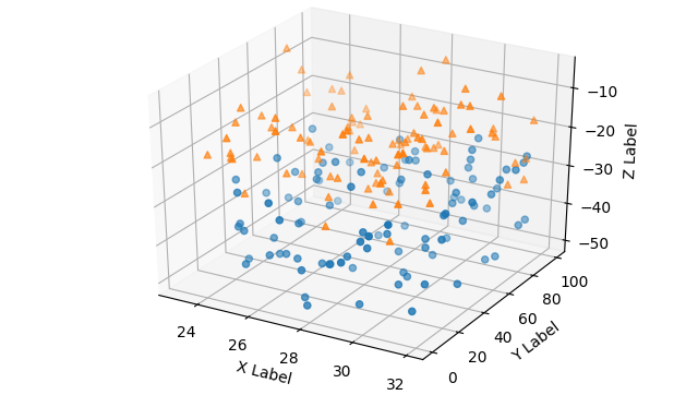
Not for me, thanks.
不适合我,谢谢。
Colour will be the third dimension here to represent data. I’ve left all columns available for the the first two columns, and just a limited selection for colours — but you can really do whatever you want.
颜色将是表示数据的第三维。 我在前两列中保留了所有列,只对颜色进行了有限的选择-但是您确实可以做任何您想做的事情。
corr_x = st.selectbox("Correlation - X variable", options=df.columns, index=df.columns.get_loc("fg3a_per_g"))
corr_y = st.selectbox("Correlation - Y variable", options=df.columns, index=df.columns.get_loc("efg_pct"))
corr_col = st.radio("Correlation - color variable", options=["age", "season", "pos_simple"], index=1)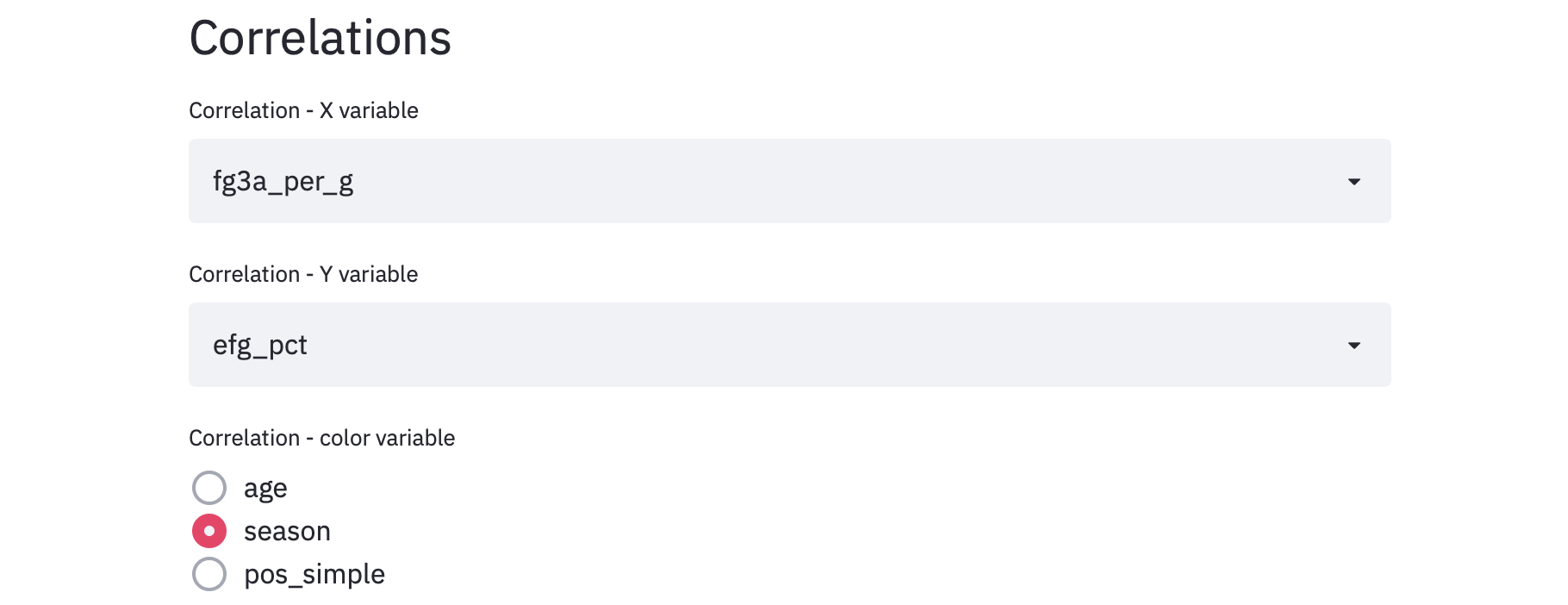
And the chart can be constructed as follows:
该图表可以构造如下:
fig = px.scatter(df, x=corr_x, y=corr_y, template="plotly_white", color=corr_col, hover_data=['name', 'pos', 'age', 'season'], color_continuous_scale=px.colors.sequential.OrRd)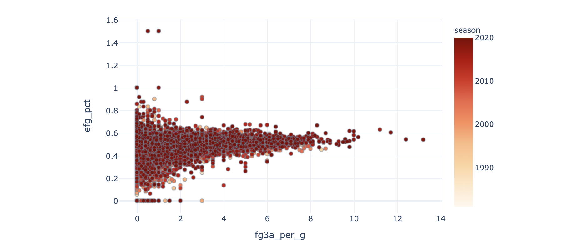
But this chart is not ideal. For one because the data is dominated by outliers. See the lonely dots on the top left? Those folks with effective FG% of 1.5 are not some gods of basketball, but it’s a side effect of extremely small sample sizes.
但是此图表并不理想。 原因之一是数据受异常值支配。 看到左上方的孤独点吗? 那些FG有效值为1.5的人不是篮球神灵,但这是极小的样本量的副作用。
So what can we do? Let’s put a filter into the data.
所以,我们能做些什么? 让我们将过滤器放入数据中。
I’m going to put in two interactive portions here, one to choose the filter parameter, and the other to put the value in. As I don’t know what the parameter is here, I will simply take an empty text box that will take numbers as inputs.
我将在此处放置两个交互式部分,一个用于选择过滤器参数,另一个用于将值放入。由于我不知道这里的参数,我将简单地使用一个空文本框以数字作为输入。
corr_filt = st.selectbox("Filter variable", options=df.columns, index=df.columns.get_loc("fg3a_per_g"))
min_filt = st.number_input("Minimum value", value=6, min_value=0)
Using these values, I can filter the dataframe like so:
使用这些值,我可以像这样过滤数据框:
tmp_df = df[df[corr_filt] > min_filt]And then pass the temporary dataframe tmp_df into the figure instead of the original dataframe, we get:
然后将临时数据帧tmp_df到图中而不是原始数据帧中,我们得到:
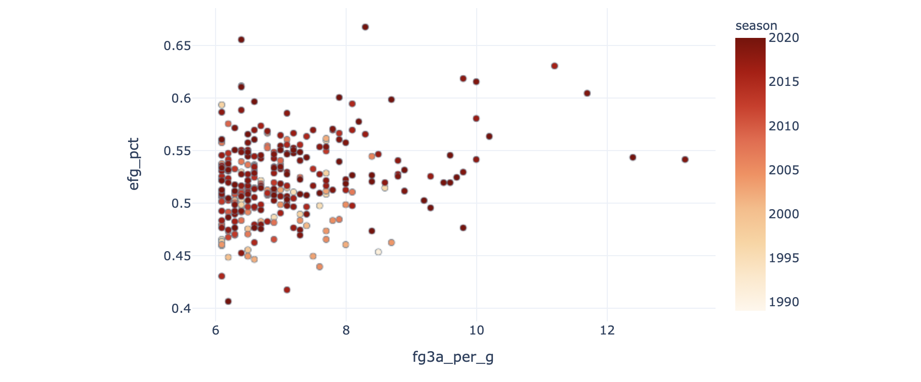
This chart could be used to take a look at correlations between various stats. For example, to see that great 3 pt shooters are also typically great free throw shooters:
该图表可用于查看各种统计数据之间的相关性。 例如,要看到出色的3分射手通常也是出色的罚球射手:

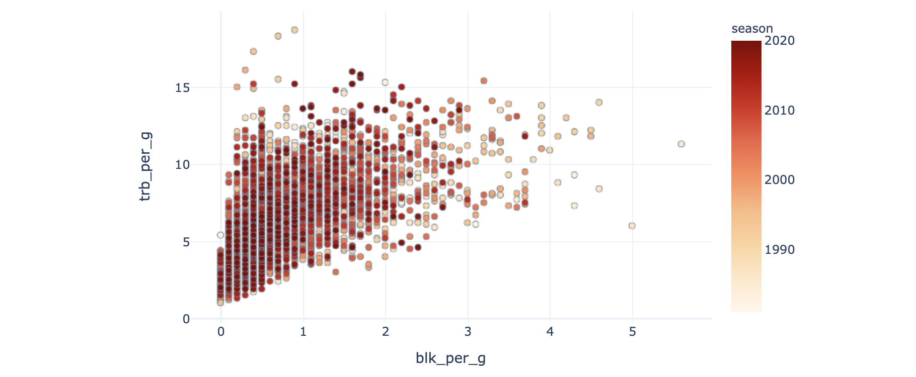
Or that great rebounders tend to be shot blockers as well. It’s also interesting that the game has changed so that no modern players average many blocks per game.
或者说,出色的篮板手也会成为盖帽手。 有趣的是,游戏发生了变化,因此没有现代玩家可以平均每场游戏获得很多积木。
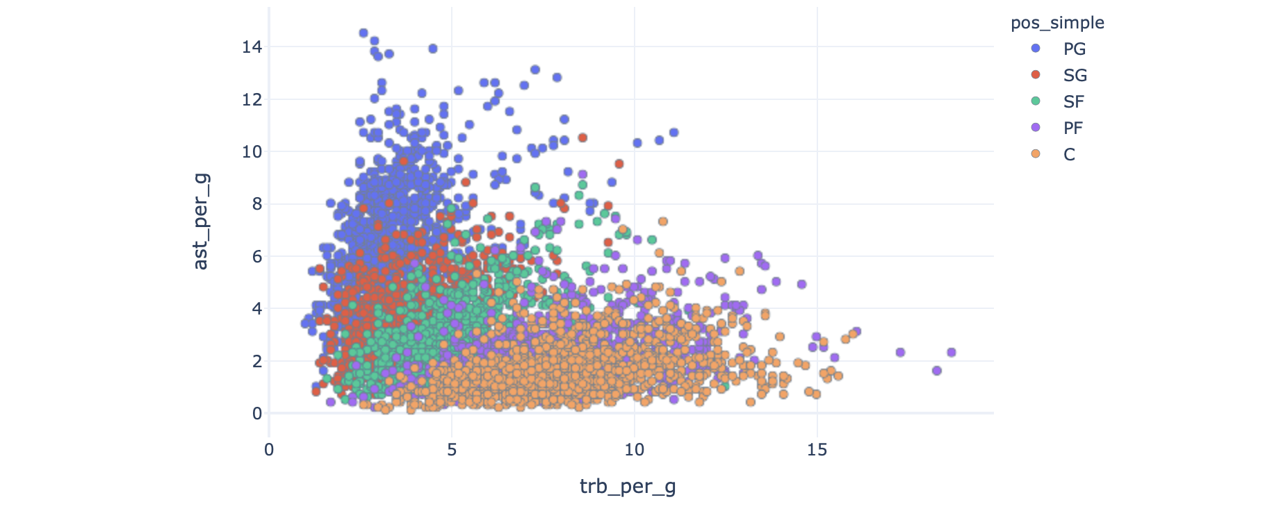
Plotting rebounds and assists, they show something of an inverse correlation, and are quite nicely stratified according to position here.
绘制篮板和助攻,它们显示出反比关系,并且根据此处的位置进行了很好的分层。
Already we can see quite a lot of trends and correlations from our app. Lastly, let’s create some heatmaps to view general correlations between sets of columns of data.
我们已经可以从我们的应用程序中看到很多趋势和相关性。 最后,让我们创建一些热图以查看数据列集之间的一般相关性。
热图的广义相关 (Generalised correlations with heatmaps)
Scatter plots are useful for seeing individual data points, but sometimes it’s good to just visualise datasets such that we can immediately see which columns might be well correlated, not correlated, or inversely correlated.
散点图对于查看单个数据点很有用,但是有时最好只是可视化数据集,这样我们就可以立即查看哪些列可能具有良好的相关性,不相关性或反相关性。
Heatmaps are perfect for this job, by setting it up to visualise what are called correlation matrices.
通过将热图设置为可视化所谓的相关矩阵,热图非常适合此工作。
Since a heatmap is best at visualising correlations between sets of input categories, let’s use an input that will take multiple categories. As a result, st.multiselect() is the module of choice here, and df.corr() is all we need to create the correlation matrix.
由于热图最适合可视化输入类别集之间的相关性,因此让我们使用将采用多个类别的输入。 结果, st.multiselect()是这里选择的模块,而df.corr()是创建相关矩阵所需的全部。
The combined code is:
组合的代码为:
hmap_params = st.multiselect("Select parameters to include on heatmap", options=list(df.columns), default=[p for p in df.columns if "fg" in p])
hmap_fig = px.imshow(df[hmap_params].corr())
st.write(hmap_fig)
And we get:
我们得到:
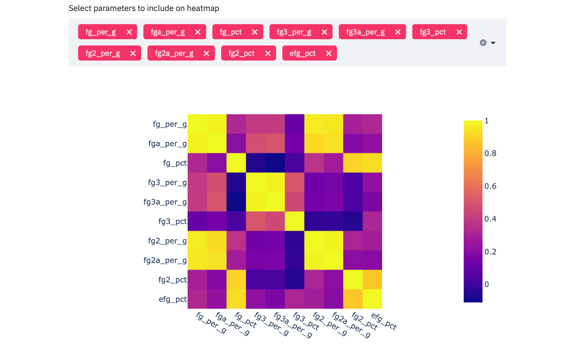
It’s so clear which of these columns are positively correlated or not correlated. and I also suggest playing with different colour scales / swatches for extra fun!
很明显,这些列中的哪一列是正相关的或不相关的。 并且我还建议您使用不同的色标/色板来获得更多的乐趣!
That’s it for today — I hope that was interesting. For my money, it’s hard to beat interactive apps like this for exploration, and the power of Plotly and Streamlit make it so easy to build these customised apps for my purpose.
今天就这样-我希望这很有趣。 为了我的钱,很难击败像这样的交互式应用程序进行探索,而Plotly和Streamlit的强大功能使为我的目的构建这些定制的应用程序变得如此容易。
And keep in mind that what I have suggested here are just basic suggestions, and what I am sure that you could build something far more useful for your own purpose and to your preference. I look forward to seeing them all!
并且请记住,我在这里提出的只是基本建议,并且我确信您可以针对自己的目的和自己的喜好构建一些更有用的东西。 我期待看到他们全部!
web数据交互


 976
976

 被折叠的 条评论
为什么被折叠?
被折叠的 条评论
为什么被折叠?
 到【灌水乐园】发言


