


jdk重启后步行
“永远不要做出预测,尤其是关于未来的预测。” (KK Steincke) (“Never Make Predictions, Especially About the Future.” (K. K. Steincke))
- Does this picture portray a horse or a car? 这张照片描绘的是马还是汽车?
- How likely is this customer to buy this item in the next week? 该客户在下周购买该商品的可能性有多大?
- Will this person fail to repay her loan over the next year? 这个人明年是否不能偿还贷款?
- How does this sentence translate to Spanish? 这句话如何翻译成西班牙语?
These questions may be answered with machine learning. But — whereas questions 1 and 4 concern things that exist already (a picture, a sentence) — questions 2 and 3 regard future events, namely events that haven’t happened yet. Is this relevant? Indeed, it is.
这些问题可以通过机器学习来回答。 但是,尽管问题1和4与已经存在的事物(一张图片,一个句子)有关,但问题2和3与未来的事件有关,即尚未发生的事件。 这相关吗? 的确是。
In fact, we all know — first as human beings, then as data scientists — that predicting the future is hard.
实际上, 我们所有人(首先是人类,然后是数据科学家)都知道,预测未来很难 。
From a technical point of view, this is due to concept drift, which is a very intuitive notion: phenomena change over time. Since the phenomenon we want to foresee is constantly changing, using a model (which learnt on the past) to predict the future poses additional challenges.
从技术角度来看,这是由于概念漂移所致,这是一个非常直观的概念:现象会随着时间而变化。 由于我们要预见的现象正在不断变化,因此使用模型(从过去学到的)来预测未来会带来更多挑战 。
In this post, I am going to describe three machine learning approaches that may be used for predicting the future, and how they deal with such challenges.
在本文中,我将描述三种可用于预测未来的机器学习方法,以及它们如何应对此类挑战。
In-Time: the approach adopted most commonly. By construction, it suffers badly from concept drift.
及时 :这种方法最常用。 通过构造,它严重遭受概念漂移的困扰。
Walk-Forward: common in some fields such as finance, but still not so common in machine learning. It overcomes some weaknesses of In-Time, but at the cost of introducing other drawbacks.
漫游 :在金融等某些领域很普遍,但在机器学习中仍然不那么普遍。 它克服了In-Time的一些弱点,但以引入其他缺点为代价。
Walk-Backward: a novel approach that combines the pros of In-Time and Walk-Forward, while mitigating their cons. I tried it on real, big, messy data and it proved to work extremely well.
向后步行 :一种新颖的方法,结合了In-Time和Walk-Forward的优点,同时减轻了它们的弊端。 我在真实,大型,混乱的数据上进行了尝试,事实证明它可以很好地工作。
In the first part of the article, we will go through the three approaches. In the second part, we will try them on data and see which one works best.
在本文的第一部分,我们将介绍三种方法。 在第二部分中,我们将在数据上对它们进行尝试,然后看看哪种方法最有效。
第一种方法:“及时” (1st Approach: “In-Time”)
Suppose today is October 1, 2020, and you want to predict the probability that the customers of your company will churn in the next month (i.e. from today to October 31).
假设今天是2020年10月1日,您想预测下个月(即从今天到10月31日)公司客户流失的可能性。
Here is how this problem is addressed in most data science projects:
以下是大多数数据科学项目中解决此问题的方法:
Note: information contained in X can go back in time indefinitely (however, in all the figures — for the sake of visual intuition — it goes back only 4 months).
注意: X中包含的信息可以无限期地返回(但是,为了直观起见,所有图中的信息只能返回4个月)。
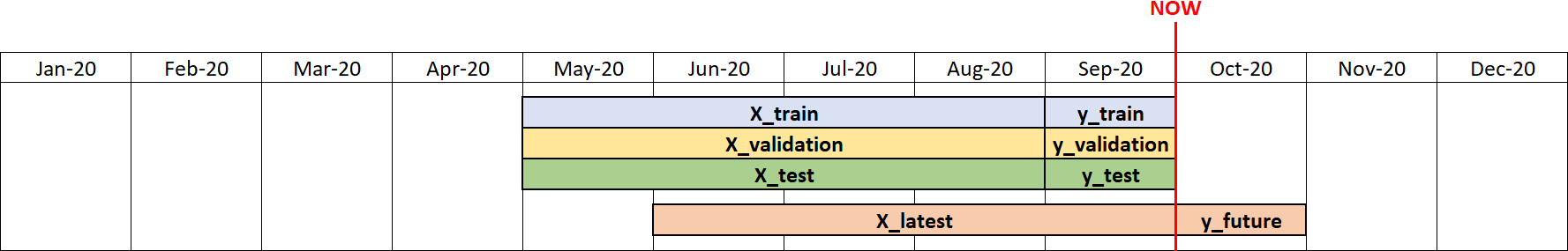
This approach is called “In-Time”, because all the datasets (train, validation and test) are taken from the same timepoint (in this case, September). By train, validation and test set, we intend:
这种方法称为“实时”,因为所有数据集(训练,验证和测试)均取自同一时间点 (在这种情况下为9月)。 通过培训,验证和测试集,我们打算:
Train set (X_train and y_train): data on which the model will learn.
训练集 ( X_train和y_train ):模型将在其上学习的数据。
Validation set (X_validation and y_validation): data used for early stopping. During the training phase, at each iteration, the validation performance is computed. When such performance stops improving, it means the model has started to overfit, so the training is arrested.
验证集 ( X_validation和y_validation ):用于提前停止的数据。 在训练阶段,每次迭代都会计算验证性能。 当这种性能停止改善时,意味着模型已经开始过拟合,因此训练被停止。
Test set (X_test and y_test): data never used during the training phase. Only used to get an estimate of how your model will actually perform in the future.
测试集 ( X_test和y_test ):在训练阶段从未使用过的数据。 仅用于估计模型将来的实际性能。
Now that you gathered the data, you fit a predictive model (let’s say an Xgboost) on the train set (September). Performance on the test set is the following: a precision of 50% with a recall of 60%. Since you are happy with this outcome, you decide to communicate this result to stakeholders and make the forecast on October.
现在,您已经收集了数据,现在可以在火车组(9月)上拟合预测模型(假设为Xgboost)。 测试仪的性能如下:精度为50%,召回率为60%。 由于您对此结果感到满意,因此您决定将此结果传达给利益相关者,并在10月进行预测。
One month later, you go and check how your model actually did in October. A nightmare. A precision of 20% with a recall of 25%. How is that possible? You did everything right. You validated your model. Then you tested it. Why do test performance and observed performance differ so drastically?
一个月后,您去检查一下您的模型在十月份的实际效果。 一个噩梦。 精度为20%,召回率为25%。 那怎么可能? 你做得对。 您验证了模型。 然后,您对其进行了测试。 为什么测试性能和观察到的性能如此巨大的差异?
过时 (Going Out-of-Time)
The problem is that concept drift is completely disregarded by the In-Time approach. In fact, this hypothesis is implicitly made:
问题在于,In-Time方法完全忽略了概念漂移。 实际上,这个假设是隐含的:

In this framework, it doesn’t really matter when the model is trained, because f(θ) is assumed to be constant over time. Unfortunately, what happens, in reality, is different. In fact, concept drift makes f(θ) change over time. In formula, this would translate to:
在此框架中, 何时训练模型并不重要,因为假设f(θ)随时间恒定。 不幸的是,实际上发生的情况是不同的。 实际上,概念漂移使f(θ)随时间变化。 在公式中,这将转换为:

To take into account this effect, we need to move our mindset from in-time to out-of-time.
要考虑到这种影响,我们需要将思维方式从及时转变为不及时。
第二种方法:“向前走” (2nd Approach: “Walk Forward”)
One form of out-of-time — mostly used in finance — is called Walk-Forward (read this article by Roger Stein to know more). This name comes from the fact that the model is validated and/or tested forward in time with respect to the data used for training. Visually:
超时的一种形式(通常用于财务)称为“向前走”(请阅读Roger Stein的这篇文章以了解更多信息)。 这个名称来自这样一个事实,即模型相对于用于训练的数据及时进行了验证和/或测试。 视觉上:
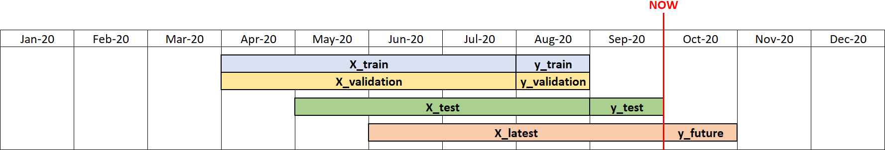
This configuration has the advantage that it simulates the real usage of the model. In fact, the model is trained on t (August), and evaluated in t+1 (September). Therefore, this is a good proxy of what can be expected by training in September and making predictions on October.
这种配置的优点是它可以模拟模型的实际用法。 实际上,该模型在t上进行了训练(8月),并在t + 1上进行了评估(9月)。 因此,这可以很好地替代9月份的培训和10月份的预测。
However, when I tried this approach on real data, I noticed it suffers from some major drawbacks:
但是,当我在真实数据上尝试这种方法时,我注意到它存在一些主要缺点:
If you use the model trained on August for making predictions on October, you would use a model which is 2-month-old! Therefore, the performance in October would be even worse than by using In-Time. Practically, this happens because the latest data is “wasted” for testing.
如果您使用8月训练的模型进行10月的预测,则将使用2个月的模型! 因此, 十月份的性能甚至比使用In-Time更差。 实际上,发生这种情况是因为“浪费”了最新数据以进行测试 。
Alternatively, if you retrain the model on September, you will fall again into In-Time. And, in the end, it will not be easy to estimate the expected performance of the model in October. So you would be back where you started.
另外, 如果您在9月对模型进行重新训练,您将再次陷入In-Time。 最后,要估计该模型在10月份的预期性能并不容易 。 因此,您将回到开始的地方。
To sum up, I liked the idea of going out-of-time, but it seemed to me that Walk-Forward was not worth it.
综上所述,我喜欢过时的想法,但在我看来,步行前进是不值得的。
第三种方法:“向后走” (3rd Approach: “Walk Backward”)
Then, this idea came to my mind: could it be that concept drift is in some way “constant” over time? In other words, could it be that predicting 1 month forward or 1 month backward leads on average to the same performance?
然后,这个想法浮现在我的脑海:难道是随着时间的推移,概念漂移在某种程度上是“恒定的”? 换句话说, 预测平均向前1个月或向后1个月会导致相同的效果吗?
If that was the case, I would have killed two birds (no, wait, three birds) with one stone. In fact, I would have kept the benefits of:
如果真是这样,我会用一块石头杀死两只鸟(不,等等,三只鸟)。 实际上,我会保留以下优势:
using the latest data for training (as happens in In-Time, but not in Walk-Forward);
使用最新的数据进行训练 (如在In-Time中进行,但在Walk-Forward中不进行);
making a reliable estimate of how the model would perform the next month (as happens in Walk-Forward, but not in In-Time);
对模型下个月的性能进行可靠的估算 (如在Walk-Forward中发生,但在In-Time中不发生);
training just one model (as happens in In-Time, but not in Walk-Forward).
仅训练一种模型 (如“实时”中那样,而在“步行”中则没有)。
In short, I would have kept the advantages of each approach, while getting rid of their drawbacks. This is how I arrived to the following configuration:
简而言之,我将保留每种方法的优点,同时消除它们的缺点。 这就是我到达以下配置的方式:
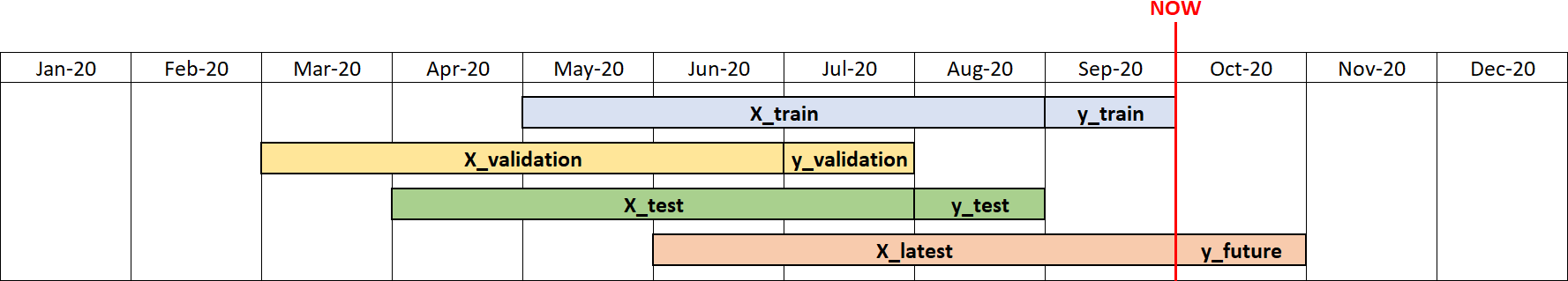
I’ve called it “Walk-Backward” because it does the exact opposite of Walk-Forward: training is made on the latest data, whereas validation and testing are made on previous time windows.
我将其称为“后退步行”,是因为它与“前进”完全相反:对最新数据进行训练,而对验证和测试则在以前的时间窗口进行。
I know it may seem crazy to train a model in September (and validate it in July), then check how it performed in August, and even expect this is a good estimate of how it will do in October! This probably looks like as if we are going back and forth in time on a DeLorean, but I promise I’ve got a good explanation.
我知道在9月训练模型(并在7月进行验证),然后检查其在8月的性能似乎疯狂,甚至期望这可以很好地估计10月的性能! 这看起来好像我们是在DeLorean上来回走动 ,但我保证我会得到很好的解释。
如果您喜欢哲学... (If You Like Philosophy…)
… then there is a philosophical explanation of why Walk-Backward makes sense. Let’s break it down.
…然后有一个哲学解释,说明为什么“后退”有意义。 让我们分解一下。
- For each set (train, validation and test), it is preferable to use a different prediction window. This is necessary to avoid that validation data or test data give a too optimistic estimate of how the model performs. 对于每组(训练,验证和测试),最好使用不同的预测窗口。 有必要避免验证数据或测试数据对模型的执行情况过于乐观。
Given point 1., training the model on September (t) is the only reasonable choice. This because the model is supposed to “learn a world” as similar as possible to the one we want to predict. And the world of September (t) is likely more similar to the world of October (t+1) than any other past month (t-1, t-2, …).
给定点1., 在9月(t)训练模型是唯一合理的选择。 这是因为该模型应该“学习一个世界”,与我们要预测的模型尽可能相似。 与过去一个月(t-1,t-2,...)相比,9月(t)的世界可能与10月(t + 1)的世界更相似。
At this point, we have a model trained on September, and would like to know how it will perform in October. Which month should be picked as test set? August is the optimal choice. In fact, the world of August (t-1) is “as different” from the world of September (t) as the world of October (t+1) is from the world of September (t). This happens for a very simple reason: October and August are equally distant from September.
至此,我们已经在9月对模型进行了训练,并且想知道它在10月的表现如何。 应该选择哪个月份作为测试集? 八月是最佳选择。 实际上,八月的世界(t-1)与九月的世界(t)“不同”,十月的世界(t + 1)与九月的世界(t)不同 。 发生这种情况的原因很简单:十月和八月与九月的距离相同。
Given points 1., 2. and 3., using July (t-2) as validation set is the only necessary consequence.
给定点1.,2和3.,使用July( t-2 )作为验证集是唯一必要的结果。
如果您不喜欢哲学... (If You Don’t Like Philosophy…)
… then, maybe, you like numbers. In that case, I can reassure you: I tried this approach on a real use-case and, compared to In-Time and Walk-Forward, Walk-Backward obtained:
……然后,也许您喜欢数字。 在那种情况下,我可以向您保证:我在一个实际用例上尝试了这种方法,并且与In-Time和Walk-Forward相比,Walk-Backward获得了:
higher precision in predicting y_future;
预测y_future的精度更高;
lower difference between performance on y_test and on y_future (i.e. the precision observed on August is a more reliable estimate of the precision that will actually obtained on October);
y_test和y_future的性能之间的差异较小 (即8月观察到的精度是对10月实际获得的精度的更可靠的估计);
lower difference between performance on y_train and on y_test (i.e. less overfitting).
y_train和y_test的性能之间的差异较小 (即,过拟合程度较低)。
Basically, everything a data scientist can ask for.
基本上,数据科学家可以要求的一切。
“我还是不相信你!” (“I Still Don’t Believe You!”)
It’s ok, I’m a skeptical guy too! This is why we will try In-Time, Walk-Foward and Walk-Backward on some data, and see which one will perform best.
没关系,我也是一个怀疑的家伙! 这就是为什么我们将对某些数据尝试In-Time,Walk-Foward和Walk-Backward,并查看哪种数据效果最好。
To do that, we will use simulated data. Simulating data is a convenient way for reproducing concept drift “in the lab” and for making the results replicable. In this way, it will be possible to check whether the superiority of Walk-Backward is confirmed in a more general setting.
为此,我们将使用模拟数据。 模拟数据是一种方便的方法,可用于“在实验室中”再现概念偏差并可以复制结果。 以这种方式,可以检查在更一般的设置中是否确认了向后走的优势。
在实验室中重现概念漂移 (Reproducing Concept Drift in the Lab)
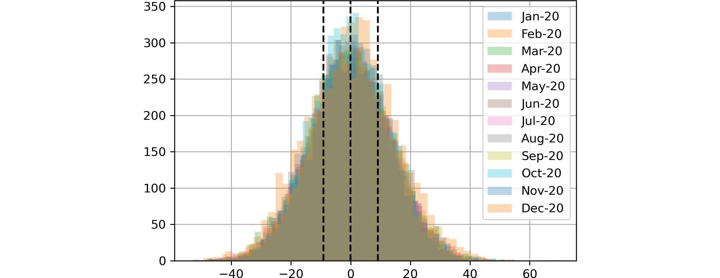
Let’s take 12 timepoints (monthly data from January 2020 to December 2020). Say that, each month, 50 features have been observed on 5,000 individuals. This means 12 dataframes (X_1, …, X_12), each one with 5,000 rows and 50 columns. To keep things simple, the columns are generated from a normal distribution:
让我们采用12个时间点(从2020年1月到2020年12月的月度数据)。 假设每个月在5,000个人身上观察到50个特征。 这意味着12个数据帧( X_1 ,…, X_12 ),每个数据帧具有5,000行和50列。 为了简单起见,这些列是从正态分布生成的:

Once X is available, we need y (dependent, or target, variable). Out of simplicity, y will be a continuous variable (but the results could be easily extended to the case in which y is discrete).
X可用后,我们需要y (因变量或目标变量)。 出于简单性考虑, y将是一个连续变量(但结果可以轻松地扩展到y是离散的情况)。
A linear relationship is assumed between X and y:
假设X和y之间存在线性关系:

βs are indexed by t because parameters change constantly over time. This is how we account for concept drift in our simplified version of the world.
βs用t索引,因为参数会随着时间不断变化。 这就是我们在简化的世界中解决概念漂移的方式 。
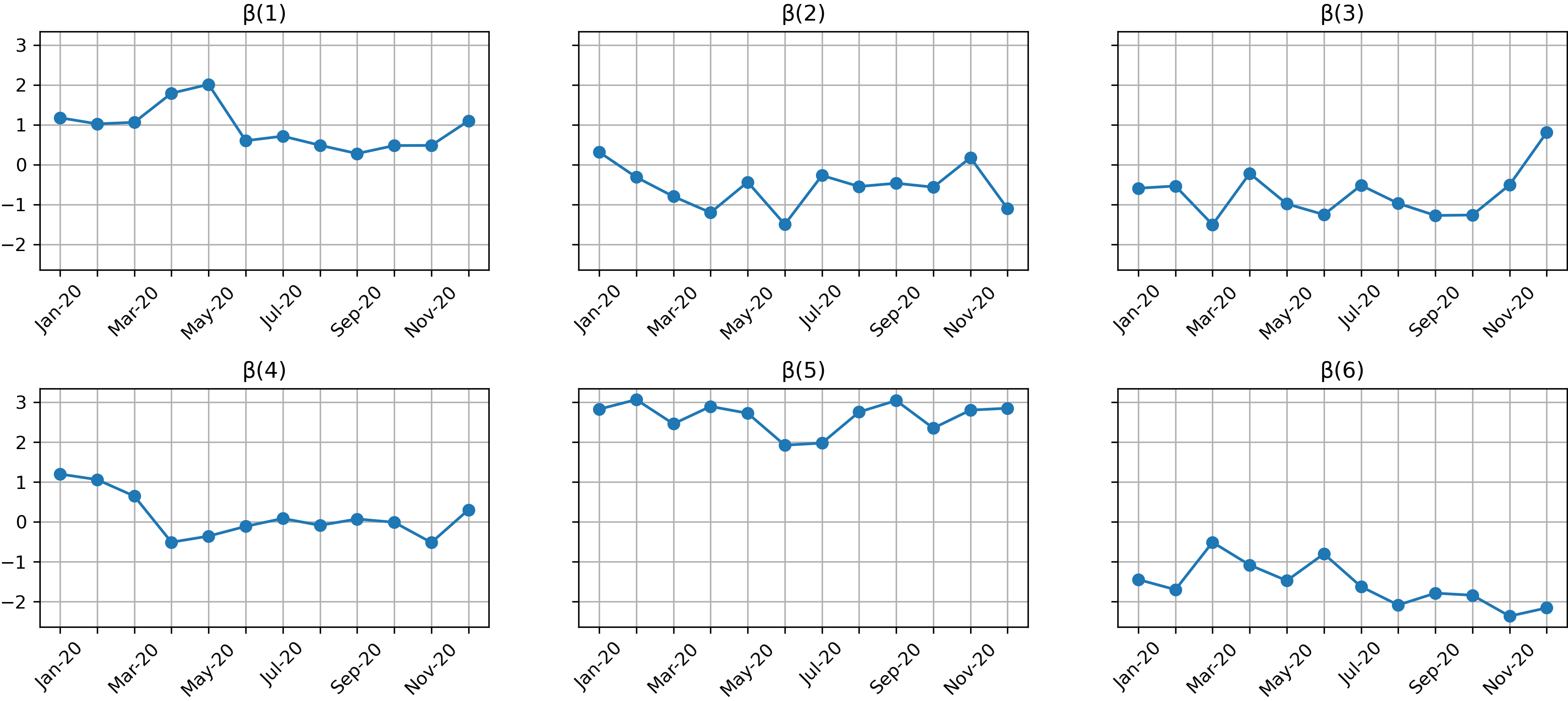
In particular, βs change according to an ARMA process. This means that the fluctuations of β(i) are not totally random: they depend on the past values of β(i) itself.
特别地, βs根据ARMA过程而变化 。 这意味着β(i)的波动并不是完全随机的:它们取决于β(i)本身的过去值。

ARMA’s coefficients (and error) are chosen based on the conservative assumption that fluctuations from month to month are not so huge (note that a more aggressive hypothesis would have favored out-of-time approaches). In particular, let’s take AR coefficient to be -0.3, MA coefficient 0.3 and standard deviation of the error 0.5. These are the resulting trajectories for the first 6 (out of 50) βs.
选择ARMA的系数(和误差)是基于一个保守的假设,即每个月的波动幅度都不大(请注意,更具攻击性的假设将有利于过时的方法)。 特别地,使AR系数为-0.3,MA系数为0.3,误差的标准偏差为0.5。 这些是前6个(总共50个) βs的合成轨迹。
And this is how the target variables (y) look like:
这就是目标变量( y )的样子:
结果 (The Outcomes)
Now that we have the data, the three approaches can be compared.
现在我们有了数据,可以比较这三种方法。
Since this is a regression problem (y is a continuous variable), mean absolute error (MAE) has been chosen as metric.
由于这是一个回归问题( y是连续变量),因此已选择平均绝对误差(MAE)作为度量。
To make the results more reliable, each approach has been carried out on all the timepoints (in a “sliding window” fashion). Then, the outcomes have been averaged over all the timepoints.
为了使结果更可靠,已在所有时间点(以“滑动窗口”方式)执行了每种方法。 然后,在所有时间点上对结果进行平均。
This is the outcome:
结果如下:
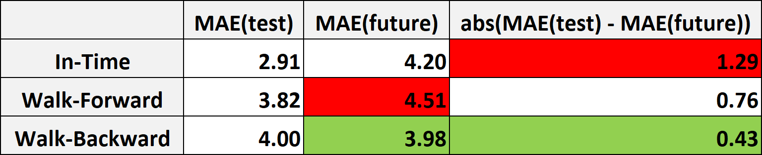
Typically, the most important indicator of a predictive model’s goodness is the performance observed on y_future. From this point of view, Walk-Backward is the best approach, since it delivers the best MAE (3.98).
通常, 预测模型优劣的最重要指标是y_future上观察到的性能。 从这个角度来看,Walk-Backward是最好的方法,因为它提供了最佳的MAE(3.98) 。
But there’s more than that. Take a look at In-Time: MAE(test) is on average 2.91, while MAE(future) is 4.20. Thus, in a real-world use case, you would communicate to stakeholders that you expect your model to deliver a MAE of 2.91. But the actual performance that you will observe one month later is on average 4.19. It’s a huge difference (and a huge disappointment)!
不仅如此。 看一下In-Time:MAE( test )平均为2.91,而MAE( future )为4.20。 因此,在实际的用例中,您将与利益相关者进行交流,您希望模型能够提供2.91的MAE。 但是一个月后您将观察到的实际性能平均为4.19。 这是一个巨大的差异(和巨大的失望)!
Indeed, the absolute difference between test performance and future performance is on average three times higher for In-Time than for Walk-Backward (1.28 versus 0.43). So, Walk-Backward turns out to be by far the best approach (also) from this perspective.
确实, In-Time的测试性能和未来性能之间的绝对差异平均比Walk-Backward高出三倍(1.28对0.43)。 因此,从这个角度来看,向后走行也是迄今为止最好的方法。
Note that, in a real-world use case, this aspect is maybe even more important than performance itself. In fact, being able to anticipate the actual performance of a model — without having to wait the end of the following period — is crucial for allocating resources and for planning actions.
请注意, 在实际的用例中,这方面可能比性能本身更为重要 。 实际上,无需等待下一个阶段的结束就能够预期模型的实际性能,这对于分配资源和计划操作至关重要。
Results are fully reproducible. Python code is available in this notebook.
结果是完全可重复的。 此笔记本中提供了Python代码。
All images created by author, through matplotlib (for plots) or codecogs (for Latex formulas).
作者通过matplotlib (用于绘图)或codecogs (用于Latex公式)创建的所有图像。
Thank you for reading! I hope you found this post useful.
感谢您的阅读! 我希望您发现这篇文章有用。
I appreciate feedback and constructive criticism. If you want to talk about this article or other related topics, you can text me at my Linkedin contact.
我感谢反馈和建设性的批评。 如果您想谈论本文或其他相关主题,可以通过Linkedin联系人发短信给我 。
jdk重启后步行


 3315
3315


 被折叠的 条评论
为什么被折叠?
被折叠的 条评论
为什么被折叠?
 到【灌水乐园】发言


