逻辑斯蒂回归 逻辑回归_从零开始了解逻辑回归

逻辑斯蒂回归 逻辑回归

表中的内容 (Table of Content)

1. Objective

1.目的

2. Load the data

2.加载数据

3. Extract features from text

3.从文本中提取特征

4. Implementation of Logistic Regression

4.逻辑回归的实现

• 4.1 Overview
  4.1概述
• 4.2 Sigmoid
  4.2乙状结肠
• 4.3 Cost function
  4.3成本函数
• 4.4 Gradient Descent
  4.4梯度下降
• 4.5 Regularization
  4.5正则化

5. Train model

5.训练模型

6. Test our logistic regression

6.测试我们的逻辑回归

7. Test with Scikit learn logistic regression

7.使用Scikit进行测试以学习逻辑回归

Let’s import all the necessary modules in Python.

让我们在Python中导入所有必需的模块。

# regular expression operations
import re    
# string operation 
import string  
# shuffle the list
from random import shuffle
# linear algebra
import numpy as np 
# data processing
import pandas as pd 
# NLP library
import nltk
# download twitter dataset
from nltk.corpus import twitter_samples                          
# module for stop words that come with NLTK
from nltk.corpus import stopwords          
# module for stemming
from nltk.stem import PorterStemmer        
# module for tokenizing strings
from nltk.tokenize import TweetTokenizer   
# scikit model selection
from sklearn.model_selection import train_test_split
# smart progressor meter
from tqdm import tqdm

1.目的 (1. Objective)

The goal of this kernel is to implement logistic regression from scratch for sentiment analysis using the twitter dataset. We will be mainly focusing on building blocks of logistic regression on our own. This kernel can provide an in-depth understanding of how logistic regression works internally. The notebook is converted to a medium article using the JupytertoMedium python library. The Kaggle notebook is available from here.

该内核的目标是使用Twitter数据集从头开始进行逻辑回归以进行情感分析。 我们将主要专注于我们自己的逻辑回归构建模块。 该内核可以深入了解逻辑回归在内部如何工作 。 使用JupytertoMedium python库将笔记本转换为中型文章。 Kaggle笔记本可从此处获得 。

Given a tweet, it will be classified if it has positive sentiment 👍 or negative sentiment 👎. It is very useful for beginners and others as well.

给定一条推文，如果它具有正面情感👍或负面情感👎 ，则将被分类。 对于初学者和其他人也非常有用。

2.加载数据 (2. Load the data)

# Download the twitter sample data from NLTK repository
nltk.download('twitter_samples')

• The twitter_samples contains 5,000 positive tweets and 5,000 negative tweets. A total of 10,000 tweets are available.

  twitter_samples包含5,000条正面推文和5,000条负面推文。 共有10,000条鸣叫。

• We have the same no of data samples in each class.
  每个类别中的数据样本数量均相同。
• It is a balanced dataset.
  它是一个平衡的数据集。

# read the positive and negative tweets
pos_tweets = twitter_samples.strings('positive_tweets.json')
neg_tweets = twitter_samples.strings('negative_tweets.json')
print(f"positive sentiment 👍 total samples {len(pos_tweets)} \nnegative sentiment 👎 total samples {len(neg_tweets)}")positive sentiment 👍 total samples 5000 
negative sentiment 👎 total samples 5000# Let's have a look at the data
no_of_tweets = 3
print(f"Let's take a look at first {no_of_tweets} sample tweets:\n")
print("Example of Positive tweets:")
print('\n'.join(pos_tweets[:no_of_tweets]))
print("\nExample of Negative tweets:")
print('\n'.join(neg_tweets[:no_of_tweets]))Let's take a look at first 3 sample tweets:

Output:

输出：

Example of Positive tweets:
#FollowFriday @France_Inte @PKuchly57 @Milipol_Paris for being top engaged members in my community this week :)
@Lamb2ja Hey James! How odd :/ Please call our Contact Centre on 02392441234 and we will be able to assist you :) Many thanks!
@DespiteOfficial we had a listen last night :) As You Bleed is an amazing track. When are you in Scotland?!
Example of Negative tweets:
hopeless for tmr :(
Everything in the kids section of IKEA is so cute. Shame I'm nearly 19 in 2 months :(
@Hegelbon That heart sliding into the waste basket. :(

• Tweets may have URLs, numbers, and special characters. Hence, we need to preprocess the text.
  推文可能包含URL，数字和特殊字符。 因此，我们需要预处理文本。

预处理文本 (Preprocess the text)

Preprocessing is one of the important steps in the pipeline. It includes cleaning and removing unnecessary data before building a machine learning model.

预处理是管道中的重要步骤之一。 它包括在建立机器学习模型之前清除和删除不必要的数据。

Preprocessing steps:

预处理步骤：

1. Tokenizing the string
   标记字符串
2. Convert the tweet into lowercase and split the tweets into tokens(words)
   将tweet转换为小写，并将tweet拆分为标记(单词)
3. Removing stop words and punctuation
   删除停用词和标点符号
4. Removing commonly used words on the twitter platform like the hashtag, retweet marks, hyperlinks, numbers, and email address
   删除Twitter平台上的常用单词，例如主题标签，转发标记，超链接，数字和电子邮件地址
5. Stemming
   抽干

• It is the process of converting a word to it’s a most general form. It helps in reducing the size of our vocabulary. Example, the word engage has different stem words like,
  这是将单词转换为最通用形式的过程。 它有助于减少我们的词汇量。 例如，engage这个词有不同的词干，例如

• engagement

  参与

• engaged

  投入

• engaging

  着迷

Let’s see how we can implement this.

让我们看看如何实现这一点。

# helper class for doing preprocessing
class Twitter_Preprocess():
    def __init__(self):
        # instantiate tokenizer class
        self.tokenizer = TweetTokenizer(preserve_case=False, strip_handles=True,
                                       reduce_len=True)
        # get the english stopwords 
        self.stopwords_en = stopwords.words('english') 
        # get the english punctuation
        self.punctuation_en = string.punctuation
        # Instantiate stemmer object
        self.stemmer = PorterStemmer() 
    def __remove_unwanted_characters__(self, tweet):
        # remove retweet style text "RT"
        tweet = re.sub(r'^RT[\s]+', '', tweet)
        # remove hyperlinks
        tweet = re.sub(r'https?:\/\/.*[\r\n]*', '', tweet)
        # remove hashtags
        tweet = re.sub(r'#', '', tweet)
        #remove email address
        tweet = re.sub('\S+@\S+', '', tweet)
        # remove numbers
        tweet = re.sub(r'\d+', '', tweet)
        ## return removed text
        return tweet
    def __tokenize_tweet__(self, tweet):        
        # tokenize tweets
        return self.tokenizer.tokenize(tweet)
    def __remove_stopwords__(self, tweet_tokens):
        # remove stopwords
        tweets_clean = []
        for word in tweet_tokens:
            if (word not in self.stopwords_en and  # remove stopwords
                word not in self.punctuation_en):  # remove punctuation
                tweets_clean.append(word)
        return tweets_clean
    def __text_stemming__(self,tweet_tokens):
        # store the stemmed word
        tweets_stem = [] 
        for word in tweet_tokens:
            # stemming word
            stem_word = self.stemmer.stem(word)  
            tweets_stem.append(stem_word)
        return tweets_stem
    def preprocess(self, tweets):
        tweets_processed = []
        for _, tweet in tqdm(enumerate(tweets)):        
            # apply removing unwated characters and remove style of retweet, URL
            tweet = self.__remove_unwanted_characters__(tweet)            
            # apply nltk tokenizer
/            tweet_tokens = self.__tokenize_tweet__(tweet)            
            # apply stop words removal
            tweet_clean = self.__remove_stopwords__(tweet_tokens)
            # apply stemmer 
            tweet_stems = self.__text_stemming__(tweet_clean)
            tweets_processed.extend([tweet_stems])
        return tweets_processed# initilize the text preprocessor class object
twitter_text_processor = Twitter_Preprocess()
# process the positive and negative tweets
processed_pos_tweets = twitter_text_processor.preprocess(pos_tweets)
processed_neg_tweets = twitter_text_processor.preprocess(neg_tweets)5000it [00:02, 2276.81it/s]
5000it [00:02, 2409.93it/s]

Let’s take a look at what output got after preprocessing tweets. It’s good that we were able to process the tweets successfully.

让我们看一下预处理推文后得到的输出。 能够成功处理这些推文是一件好事。

pos_tweets[:no_of_tweets], processed_pos_tweets[:no_of_tweets](['#FollowFriday @France_Inte @PKuchly57 @Milipol_Paris for being top engaged members in my community this week :)',
  '@Lamb2ja Hey James! How odd :/ Please call our Contact Centre on 02392441234 and we will be able to assist you :) Many thanks!',
  '@DespiteOfficial we had a listen last night :) As You Bleed is an amazing track. When are you in Scotland?!'],
 [['followfriday', 'top', 'engag', 'member', 'commun', 'week', ':)'],
  ['hey',
   'jame',
   'odd',
   ':/',
   'pleas',
   'call',
   'contact',
   'centr',
   'abl',
   'assist',
   ':)',
   'mani',
   'thank'],
  ['listen', 'last', 'night', ':)', 'bleed', 'amaz', 'track', 'scotland']])

3.从文本中提取特征 (3. Extract features from text)

• Given the text, It is very important to represent features (numeric values) such a way that we can feed into the model.

  给定文本，以能够馈入模型的方式来表示features (numeric values)非常重要。

3.1创建单词袋(BOW)表示形式 (3.1 Create a Bag Of Words (BOW) representation)

BOW represents the word and its frequency for each class. We will create a dict for storing the frequency of positive and negative classes for each word.Let’s indicate a positive tweet is 1 and the negative tweet is 0. The dict key is a tuple containing the(word, y) pair. The word is processed word and y indicates the label of the class. The dict value represents the frequency of the word for class y.

BOW代表每个类别的单词及其出现的频率。 我们将创建一个dict来存储每个单词的positive和negative类别的频率。让我们指出一个positive推文是1和negative推文是0 。 dict键是一个包含(word, y)对的元组。 该word为已处理单词， y表示类别的标签。 dict值表示y类frequency of the word的frequency of the word 。

Example: #word bad occurs 45 time in the 0 (negative) class {(“bad”, 0) : 32}

示例：#word错误在0(负)类{(“ bad”，0)：32}中出现45次

# word bad occurs 45 time in the 0 (negative) class 
{("bad", 0) : 45}# BOW frequency represent the (word, y) and frequency of y class
def build_bow_dict(tweets, labels):
    freq = {}
    ## create zip of tweets and labels
    for tweet, label in list(zip(tweets, labels)):
        for word in tweet:
            freq[(word, label)] = freq.get((word, label), 0) + 1
    return freq# create labels of the tweets
# 1 for positive labels and 0 for negative labels
labels = [1 for i in range(len(processed_pos_tweets))]
labels.extend([0 for i in range(len(processed_neg_tweets))])
# combine the positive and negative tweets
twitter_processed_corpus = processed_pos_tweets + processed_neg_tweets
# build Bog of words frequency 
bow_word_frequency = build_bow_dict(twitter_processed_corpus, labels)

Now, we have various methods to represent features for our twitter corpus. Some of the basic and powerful techniques are,

现在，我们有多种方法来表示Twitter语料库的功能。 一些基本而强大的技术是

• CountVectorizer
  CountVectorizer
• TF-IDF feature
  TF-IDF功能

1. CountVectorizer (1. CountVectorizer)

The count vectorizer indicates the sparse matrix and the value can be the frequency of the word. Each column is a unique token in our corpus.

计数矢量化器指示稀疏矩阵，其值可以是单词的频率 。 每列都是我们语料库中的唯一标记。

The sparse matrix dimension would be no of unique tokens in the corpus * no of sample tweets.

稀疏矩阵维将是no of unique tokens in the corpus * no of sample tweets 。

Example: corpus = [ 'This is the first document.', 'This document is the second document.', 'And this is the third one.', 'Is this the first document?', ] and the CountVectorizer representation is

示例： corpus = [ 'This is the first document.', 'This document is the second document.', 'And this is the third one.', 'Is this the first document?', ] ，CountVectorizer表示为

[[0 1 1 1 0 0 1 0 1] [0 2 0 1 0 1 1 0 1] [1 0 0 1 1 0 1 1 1] [0 1 1 1 0 0 1 0 1]]

[[0 1 1 1 0 0 1 0 1] [0 2 0 1 0 1 1 0 1] [1 0 0 1 1 0 1 1 1] [0 1 1 1 0 0 1 0 1]]

2. TF-IDF(术语频率-反向文档频率) (2. TF-IDF (Term Frequency — Inverse Document Frequency))

TF-IDF statistical measure that evaluates how relevant a word is to a document in a collection of documents. TF-IDF is computed as follows:

TF-IDF统计量度，用于评估单词与文档集中的文档的相关性。 TF-IDF的计算如下：

TF-IDF equation

TF-IDF方程

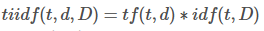
Term Frequency: term frequency tf(t,d), the simplest choice is to use the frequency of a term (word) in a document. Inverse Document Frequency: idf(t,D) a measure of how much information the word provides, i.e., if it’s common or rare across all documents. It is the logarithmic scale of the inverse fraction of the document that contains the word. The definition is as per Wiki.

术语频率：术语频率tf(t，d) ，最简单的选择是使用文档中术语(单词)的频率。 反向文档频率： idf(t，D)衡量单词提供多少信息的度量，即，该单词在所有文档中是常见还是罕见。 它是包含单词的文档反分数的对数标度 。 定义根据Wiki 。

3.2。 为我们的模型提取简单特征 (3.2. Extracting simple features for our model)

• Given a list of tweets, we will be extracting two features.
  给定一系列推文，我们将提取两个功能。
• The first feature is the number of positive words in a tweet.
  第一个功能是一条推文中肯定词的数量。
• The second feature is the number of negative words in a tweet.
  第二个特征是一条推文中否定词的数量。

This seems to be simple, isn’t it? Perhaps yes. We are not representing our features to the sparse matrix. Will use the simplest features for our analysis.

这似乎很简单，不是吗？ 也许是。 我们没有将特征表示为稀疏矩阵。 将使用最简单的功能进行分析。

# extract feature for tweet
def extract_features(processed_tweet, bow_word_frequency):
    # feature array
    features = np.zeros((1,3))
    # bias term added in the 0th index
    features[0,0] = 1
    # iterate processed_tweet
    for word in processed_tweet:
        # get the positive frequency of the word
        features[0,1] = bow_word_frequency.get((word, 1), 0)
        # get the negative frequency of the word
        features[0,2] = bow_word_frequency.get((word, 0), 0)
    return features

Shuffle the corpus and will split the train and test set.

改编语料，将火车和测试仪分开。

# shuffle the positive and negative tweets
shuffle(processed_pos_tweets)
shuffle(processed_neg_tweets)
# create positive and negative labels
positive_tweet_label = [1 for i in processed_pos_tweets]
negative_tweet_label = [0 for i in processed_neg_tweets]
# create dataframe
tweet_df = pd.DataFrame(list(zip(twitter_processed_corpus, positive_tweet_label+negative_tweet_label)), columns=["processed_tweet", "label"])

3.3训练和测试拆分 (3.3 Train and Test split)

Let’s keep the 80% data for training and 20% data samples for testing.

让我们保留用于训练的80％数据和用于测试的20％数据样本。

# train and test split
train_X_tweet, test_X_tweet, train_Y, test_Y = train_test_split(tweet_df["processed_tweet"], tweet_df["label"], test_size = 0.20, stratify=tweet_df["label"])
print(f"train_X_tweet {train_X_tweet.shape}, test_X_tweet {test_X_tweet.shape}, train_Y {train_Y.shape}, test_Y {test_Y.shape}")train_X_tweet (8000,), test_X_tweet (2000,), train_Y (8000,), test_Y (2000,)# train X feature dimension
train_X = np.zeros((len(train_X_tweet), 3))
for index, tweet in enumerate(train_X_tweet):
    train_X[index, :] = extract_features(tweet, bow_word_frequency)
# test X feature dimension
test_X = np.zeros((len(test_X_tweet), 3))
for index, tweet in enumerate(test_X_tweet):
    test_X[index, :] = extract_features(tweet, bow_word_frequency)
print(f"train_X {train_X.shape}, test_X {test_X.shape}")train_X (8000, 3), test_X (2000, 3)

Output:

输出：

train_X[0:5]array([[1.000e+00, 6.300e+02, 0.000e+00],
       [1.000e+00, 6.930e+02, 0.000e+00],
       [1.000e+00, 1.000e+00, 4.570e+03],
       [1.000e+00, 1.000e+00, 4.570e+03],
       [1.000e+00, 3.561e+03, 2.000e+00]])

Take a look at sample train features.

看一下样本火车功能。

• The 0th index is a bias term added.
  第0个索引是添加的偏差项。
• 1st index is representing positive word frequency
  第一个索引代表正词频
• 2nd index is representing negative word frequency
  第二个索引代表负词频率

4.逻辑回归的实现 (4. Implementation of Logistic Regression)

4.1概述 (4.1 Overview)

Now, Let’s see how logistic regression works and gets implemented.

现在，让我们看看逻辑回归是如何工作和实现的。

Most of the time, when you hear about logistic regression you may think, it is a regression problem. No, it is not, Logistic regression is a classification problem and it is a non-linear model.

大多数时候，当您听说逻辑回归时，您可能会认为这是一个回归问题。 不，不是， 逻辑回归是一个分类问题，它是一个非线性模型。

Created by Author

由作者创建

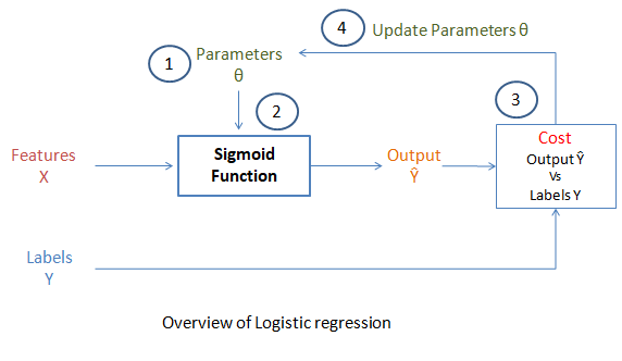
As shown in the above picture, there are 4 stages for most of the ML algorithms,

如上图所示，大多数ML算法有4个阶段，

Step 1. Initialize the weights

步骤1.初始化权重

• Random weights initialized
  随机权重已初始化

Step 2. Apply function

步骤2.应用功能

• Calculate the sigmoid
  计算S形

Step 3. Calculate the cost (objective of the algorithm)

步骤3.计算成本(算法的目标)

• Calculate the log-loss for binary classification
  计算二进制分类的对数损失

Step 4. Gradient Descent

步骤4.梯度下降

• Update the weights iteratively till finding the minimum cost
  迭代更新权重，直到找到最低成本

Logistic regression takes a linear regression and applies a sigmoid to the output of the linear regression. So, It produces the probability of each class and it sums up to 1.

Logistic回归采用线性回归，然后将S型线应用于线性回归的输出。 因此，它产生每个类别的概率，总和为1。

Regression: Single linear regression equation as follows:

回归：单个线性回归方程如下：

Single variable Linear regression formula

单变量线性回归公式

• Note that the theta values are weights

  注意theta值是权重

• x_0, x_1, x_2,… x_N is input features

  x_0，x_1，x_2 ...…x_N是输入要素

You may think of how complicated the equation it is. We need to multiply all the weighs with each feature at the ith position then sums up all.

您可能会想到方程式有多复杂。 我们需要将所有权重与每个特征的ith位置相乘，然后求和。

Fortunately, Linear algebra brings this equation with ease of operation. Yes, It is a matrix dot product. You can apply the dot product of features and weights to find the z.

幸运的是， 线性代数使该方程式易于操作。 是的，它是矩阵dot积。 您可以应用特征和权重的点积来找到z 。

4.2乙状结肠 (4.2 Sigmoid)

• The sigmoid function is defined as:
  乙状结肠功能定义为：

Sigmoid function 乙状结肠功能

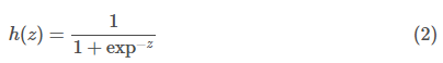
It maps the input ‘z’ to a value that ranges between 0 and 1, and so it can be treated as a probability.

它将输入“ z”映射到介于0和1之间的值，因此可以将其视为概率 。

def sigmoid(z): 
    # calculate the sigmoid of z
    h = 1 / (1+ np.exp(-z))
    return h

4.3成本函数 (4.3 Cost function)

The cost function used in logistic regression is:

逻辑回归中使用的成本函数为：

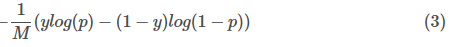
This is the Log loss of binary classification. The average of the log loss across all training samples is calculated in logistic regression, the equation 3 modified for all the training samples as follows:

这是二进制分类的对数丢失。 所有训练样本的对数损失平均值通过对数回归进行计算，对所有训练样本的等式3进行了如下修改：

• m is the number of training examples

  m是训练示例数

• y^{(i)} is the actual label of the ith training example.

  y ^ {(i)}是第i个训练示例的实际标签。

• h(z(\theta)^{(i)}) is the model’s prediction for the ith training example.

  h(z(\ theta)^ {(i)})是第i个训练示例的模型预测。

The loss function for a single training example is,

单个训练示例的损失函数为

Loss function

损失函数

• All the h values are between 0 and 1, so the logs will be negative. That is the reason for the factor of -1 applied to the sum of the two loss terms.

  所有的h 值介于0和1之间，因此对数将为负。 这就是将因子-1应用于两个损失项之和的原因。

• When the model predicts 1, (h(z(θ))=1) and the label y is also 1, the loss for that training example is 0.

  当模型预测1时，( h ( z ( θ ))= 1)和标签y 也为1，则该训练示例的损失为0。

• Similarly, when the model predicts 0, (h(z(θ))=0) and the actual label is also 0, the loss for that training example is 0.

  类似地，当模型预测为0(( h ( z ( θ ))= 0)并且实际标签也为0时，该训练示例的损失为0。

• However, when the model prediction is close to 1 (h(z(θ))=0.9999) and the label is 0, the second term of the log loss becomes a large negative number, which is then multiplied by the overall factor of -1 to convert it to a positive loss value. −1×(1−0)×log(1−0.9999)≈9.2 The closer the model prediction gets to 1, the larger the loss.

  但是，当模型预测接近1( h ( z ( θ ( θ ))= 0.9999)且标签为0时，对数损失的第二项变为较大的负数，然后将其乘以-的总因数1将其转换为正损耗值。 -1×(1-0)× log (1-0.9999)≈9.2模型预测值越接近1，则损失越大。

4.4梯度下降 (4.4 Gradient Descent)

Gradient Descent is an algorithm used for updating the weights theta iteratively to minimize the objective function (cost). We need to update the weights iteratively because,

梯度下降是一种用于迭代更新权重以最小化目标函数(成本)的算法。 我们需要迭代更新权重，因为，

At initial random weights, the model doesn’t learn anything much. To improve the prediction we need to learn from the data with multiple iterations and tune the random weights accordingly.

在初始随机权重下，模型不会学到很多东西。 为了改善预测，我们需要通过多次迭代从数据中学习并相应地调整随机权重。

The gradient of the cost function J for one of the weights theta_j is:

权重theta_j之一的成本函数J的梯度为：

gradient function

梯度函数

4.5正则化 (4.5 Regularization)

Regularization is a technique to solve the problem of overfitting in a machine learning algorithm by penalizing the cost function. There will be an additional penalty term in the cost function. There are two types of regularization techniques:

正则化是一种通过惩罚成本函数来解决机器学习算法过拟合问题的技术。 成本函数中将有一个附加的惩罚项。 有两种类型的正则化技术：

• Lasso (L1-norm) Regularization
  套索(L1-范数)正则化
• Ridge (L2-norm) Regularization
  岭(L2-范数)正则化

Lasso Regression (L1) L1-norm loss function is also known as the least absolute errors (LAE). $λ*∑ |w| $ is a regularization term. It is a product of $λ$ regularization term with an absolute sum of weights. The smaller values indicate stronger regularization.

套索回归(L1) L1范数损失函数也称为最小绝对误差(LAE)。 $λ* ∑ | w | $是正则项。 它是$λ$正则化项与绝对权重之和的乘积。 较小的值表示更强的正则化。

Ridge Regression (L2) L2-norm loss function is also known as the least squares error (LSE). $λ*∑ (w)²$ is a regularization term. It is a product of $λ$ regularization term with the squared sum of weights. The smaller values indicate stronger regularization.

岭回归(L2) L2范数损失函数也称为最小二乘误差(LSE)。 $λ* ∑(w)²$是正则项。 它是$λ$正则化项与权重平方和的乘积。 较小的值表示更强的正则化。

You could notice, that it makes a huge difference. Yes, it does well. The main difference is what type of regularization term you are adding in the cost function to minimize the error.

您可能会注意到，这有很大的不同。 是的，它做得很好。 主要区别在于您要在成本函数中添加哪种类型的正则化项以最大程度地减少误差。

L2 (Ridge) shrinks all the coefficient by the same proportions but it doesn’t eliminate any features, while L1 (Lasso) can shrink some coefficients to zero, and also performs feature selection.

L2(Ridge)将所有系数按相同比例缩小，但不会消除任何特征，而L1(Lasso)可以将某些系数缩小到零，并执行特征选择。

In the following code will add L2 regularization

在下面的代码中将添加L2正则化

# implementation of gradient descent algorithm  def gradientDescent(x, y, theta, alpha, num_iters, c):    # get the number of samples in the training
    m = x.shape[0]
    for i in range(0, num_iters):
        # find linear regression equation value, X and theta
        z = np.dot(x, theta)
        # get the sigmoid of z
        h = sigmoid(z)
        # calculate the cost function, log loss
        #J = (-1/m) * (np.dot(y.T, np.log(h)) + np.dot((1 - y).T, np.log(1-h)))
        # let's add L2 regularization
        # c is L2 regularizer term
        J = (-1/m) * ((np.dot(y.T, np.log(h)) + np.dot((1 - y).T, np.log(1-h))) + (c * np.sum(theta)))
        # update the weights theta
        theta = theta - (alpha / m) * np.dot((x.T), (h - y))
    J = float(J)
    return J, theta

5.训练模型 (5. Train model)

Let’s train the gradient descent function for optimizing the randomly initialized weights. The brief explanation has given in section 4.

让我们训练梯度下降函数以优化随机初始化的权重。 简要说明在第4节中给出。

# set the seed in numpy
np.random.seed(1)
# Apply gradient descent of logistic regression
# 0.1 as added L2 regularization term
J, theta = gradientDescent(train_X, np.array(train_Y).reshape(-1,1), np.zeros((3, 1)), 1e-7, 1000, 0.1)
print(f"The cost after training is {J:.8f}.")
print(f"The resulting vector of weights is {[round(t, 8) for t in np.squeeze(theta)]}")The cost after training is 0.22154867.
The resulting vector of weights is [2.18e-06, 0.00270863, -0.00177371]

6.测试我们的逻辑回归 (6. Test our logistic regression)

It is time to test our logistic regression function on test data that the model has not seen before.

现在该对模型从未见过的测试数据测试逻辑回归函数了。

Predict whether a tweet is positive or negative.

预测一条推文是肯定的还是负面的。

• Apply the sigmoid to the logits to get the prediction (a value between 0 and 1).
  将S形应用于logit以获得预测(0到1之间的值)。

Prediction for new tweets

新推文的预测

# predict for the features from learned theata values
def predict_tweet(x, theta):
    # make the prediction for x with learned theta values
    y_pred = sigmoid(np.dot(x, theta))
    return y_pred# predict for the test sample with the learned weights for logistics regression
predicted_probs = predict_tweet(test_X, theta)
# assign the probability threshold to class
predicted_labels = np.where(predicted_probs > 0.5, 1, 0)
# calculate the accuracy
print(f"Own implementation of logistic regression accuracy is {len(predicted_labels[predicted_labels == np.array(test_Y).reshape(-1,1)]) / len(test_Y)*100:.2f}")Own implementation of logistic regression accuracy is 93.45

As of now, we have seen how to implement the logistic regression on our own. Got the accuracy of 94.45. Let’s see the results from the popular Machine Learning (ML) Python library.

到目前为止，我们已经看到了如何独自实现逻辑回归。 获得了94.45的准确性。 让我们看看流行的机器学习(ML)Python库的结果。

7.使用Scikit进行测试以学习逻辑回归 (7. Test with Scikit learn logistic regression)

Here, we are going to train the logistic regression from the in-build Python library to check the results.

在这里，我们将训练内置Python库中的逻辑回归以检查结果。

# scikit learn logiticsregression and accuracy score metric
from sklearn.linear_model import LogisticRegression
from sklearn.metrics import accuracy_score
clf = LogisticRegression(random_state=42, penalty='l2')
clf.fit(train_X, np.array(train_Y).reshape(-1,1))
y_pred = clf.predict(test_X)/opt/conda/lib/python3.7/site-packages/sklearn/utils/validation.py:73: DataConversionWarning: A column-vector y was passed when a 1d array was expected. Please change the shape of y to (n_samples, ), for example using ravel().
  return f(**kwargs)print(f"Scikit learn logistic regression accuracy is {accuracy_score(test_Y , y_pred)*100:.2f}")Scikit learn logistic regression accuracy is 94.45

Great!!!. The results are pretty much close.

大！！！。 结果非常接近。

Finally, we implemented the logistic regression on our own and also tried with in-build Scikit learn logistic regression getting similar accuracy. But, this approach of feature extraction is very simple and intuitive.

最后，我们自己实现了逻辑回归，还尝试使用内置Scikit学习逻辑回归来获得相似的准确性。 但是，这种特征提取方法非常简单直观。

I am learning by doing it. Kindly leave your thoughts or any suggestions in the comments. Your feedback is highly appreciated to boost my confidence.

我正在这样做。 请在评论中留下您的想法或任何建议。 非常感谢您的反馈，以增强我的信心。

🙏Thanks for reading! You can reach me via LinkedIn.

🙏感谢您的阅读！ 您可以通过LinkedIn与我联系。

翻译自: https://towardsdatascience.com/understand-logistic-regression-from-scratch-430aedf5edb9

逻辑斯蒂回归 逻辑回归