具有keras的图像分类器

I have recently graduated from university this summer in the midst of the current global situation (big ups to Class of 2020!), and for my Artificial Intelligence module, I had to create an image classifier that would be able to classify fruits & vegetables. In this article, I will show you how to create your own Convolutional Neural Network (CNN) and I will explain every step I took to successfully complete my AI project.

我最近已于今年夏天从当前全球形势中大学毕业(到2020级！)。对于我的人工智能模块，我必须创建一个图像分类器，以便对水果和蔬菜进行分类。 在本文中，我将向您展示如何创建自己的卷积神经网络(CNN)，并说明成功完成AI项目所采取的每一步。

创建工作区 (Creating the workspace)

I used Google Colab, a cloud-based environment similar to Jupyter Notebook, to create a notebook which would contain all the code for the project. After creating the notebook, I then changed the notebook’s settings by setting the Hardware Accelerator to GPU, which can be done by clicking on Edit and then Notebook settings. It will also be nice if you create a folder on your desktop that will be used later, in which you will import and export files to e.g. image_classifier. If you want to code along, I’d advise you start your runtime now and run each cell as we go, or you can just Run All cells at the end.

我使用Google Colab(一种类似于Jupyter Notebook的基于云的环境)来创建一个笔记本，其中将包含项目的所有代码。 创建笔记本之后，我通过将Hardware Accelerator设置为GPU来更改笔记本的设置，这可以通过单击Edit ，然后单击Notebook settings来完成。 如果您在桌面上创建一个文件夹供以后使用，也可以将其导入和导出到例如 image_classifier ，这也很好 。 如果您想进行编码，建议您立即开始运行，并在运行时运行每个单元，或者最后只运行所有单元。

导入数据集和所需的包 (Importing the dataset and required packages)

To import the dataset we will be using, you will have to register an account on Kaggle. Once your Kaggle account has been created, access the My Account page and scroll down until you see the API section. Click the Create New API Token, which should generate a Kaggle file that you can save into the folder that we created earlier. Now that we have the API token in our image_classifier directory, we can now start working on our project! (*inserts everybody say yeah meme*)

要导入我们将使用的数据集，您必须在Kaggle上注册一个帐户。 创建Kaggle帐户后，访问“我的帐户”页面并向下滚动，直到看到“ API”部分。 点击创建新API令牌 ，这将生成一个Kaggle文件，您可以将其保存到我们之前创建的文件夹中。 现在我们在image_classifier目录中有了API令牌，现在我们可以开始处理我们的项目了！ (*插入所有人都说是对的模因*)

Kaggle API section

Kaggle API部分

Next, place the following in your code cell. We will be separating the code into different cells to be able to identify errors better. This will allow you to import the API token we obtained earlier into the workspace when we run all cells at a later time. This is my personal preferred approach, as it will allow us to download the dataset through the notebook, without having to download the dataset to our local area and then upload it to the notebook.

接下来，将以下内容放入您的代码单元中。 我们将把代码分成不同的单元，以便能够更好地识别错误。 这将允许您在稍后运行所有单元时将先前获得的API令牌导入工作空间。 这是我个人首选的方法，因为它将允许我们通过笔记本电脑下载数据集，而不必将数据集下载到我们的本地区域然后再将其上传到笔记本电脑。

# import files
files.upload()

To make it easier to follow and so I don’t repeat myself a lot, I’d advise you create a new code cell per code snippet you see from now on. Create a new code cell and let’s modify the permissions of the API file.

为了更容易理解，在此我不再赘述，我建议您从现在开始为每个代码段创建一个新的代码单元。 创建一个新的代码单元，让我们修改API文件的权限。

# modifying the permission of the kaggle file!mkdir -p ~/.kaggle!cp kaggle.json ~/.kaggle/!chmod 600 ~/.kaggle/kaggle.jsonprint('[INFO] API token permission modified!')

Next, we will be downloading the Fruits 360 dataset on Kaggle by Mihai Oltean. The print statements will allows us to see everything that is happening and provide some output to us like a terminal.

接下来，我们将在Mihai Oltean的Kaggle上下载Fruits 360数据集。 打印语句将使我们能够看到正在发生的一切，并像终端一样向我们提供一些输出。

# downloading the dataset!kaggle datasets download -d moltean/fruitsprint('[INFO] dataset downloaded!')

Now, we will extract the contents from the zipped dataset we have just downloaded.

现在，我们将从刚刚下载的压缩数据集中提取内容。

# extracting the contents of the zipped dataset from the kaggle source!unzip -q fruits.zip
print('[INFO] dataset unzipped!')

We have our dataset ready, let’s import the required packages!

我们已经准备好数据集，让我们导入所需的包！

# importing required packagesfrom keras import * # importing everything from keras (mainly for the Keras models, layers etc...)from keras.applications.vgg19 import VGG19, preprocess_input # importing the pretrained modelimport datetime # to calculate the training durationimport os # to operate with the file system of the projectimport pandas as pd # to be used along the confusion matriximport seaborn as sn # to be used along the confusion matrixfrom imutils import paths # to operate with the path structure of the projectimport matplotlib.pyplot as plt # to plot the results over the given training durationfrom sklearn.metrics import confusion_matrix, classification_report # to produce a confusion matrixfrom keras.preprocessing.image import ImageDataGenerator # to preprocess the image data before feeding it into the modelfrom numpy import argmax # to return the indices in max element in an array (used in the confusion matrix)

设置培训和测试目录 (Setting up the Training and Test directories)

Before we go any further, make sure that the contents of the zipped file have been extracted completely. Click the folder icon on the left panel, and check that the Fruits-360 folder shows all the classes available and their samples.

在继续进行之前，请确保已完全提取压缩文件的内容。 单击左侧面板上的文件夹图标，然后检查Fruits-360文件夹是否显示了所有可用的类及其示例。

The following code snippet will locate the Training and Test directories from the dataset and also check the number of classes in the dataset, as the dataset is updated often. Using len(labels) will also help us later, as it will place the number of classes automatically by reading the number of folders in the training directory, without us having to count the amount of subdirectories under the Training folder.

以下代码段将从数据集中找到Training和Test目录，并检查数据集中的类数，因为数据集经常更新。 使用len(labels)以后也会对我们有帮助，因为它将通过读取培训目录中的文件夹数量自动放置类的数量，而无需我们计算培训文件夹下的子目录数量。

# locating the training directory
train_path = '/content/fruits-360/Training'# locating the testing directory
test_path = '/content/fruits-360/Test'use_label_file = False  # this will be set to true if the label names from a file are to be loaded; it uses the label_file defined below; the file should contain the names of the used labels on a separate linelabel_file = 'labels.txt'output_dir = 'output_files'if not os.path.exists(output_dir):
   os.makedirs(output_dir)if use_label_file:
   with open(label_file, "r") as f:
     labels = [x.strip() for x in f.readlines()]else:
   labels = os.listdir(train_path)# prints the names of all classes
print(labels)# prints the number of classes available
len(labels)

样品检查 (Sample Checking)

This is essentially checking the number of samples in the Training and Test folders. This can be useful for when we perform a validation split — remember this for later.

这实际上是检查“训练”和“测试”文件夹中的样本数量。 当我们执行验证拆分时，这可能很有用-请稍后记住。

# directoriestotalTrain = len(list(paths.list_images(train_path)))totalTest = len(list(paths.list_images(test_path)))total = totalTrain + totalTest# outputprint("[INFO] There are "+str(totalTrain)+ " samples in the Train path")print("[INFO] There are "+str(totalTest)+ " samples in the Test path")print("[INFO] There are a total of "+str(total)+ " samples")

设置全局参数和功能 (Setting Global Parameters and Functions)

Let’s set up the global parameters. These global parameters allow for easier modification if you want to use different values, like a different optimizer and learning rate. This code snippet does the following: sets the image_size variable to 100 because each image is 100 by 100 pixels big, the batch_size will take 128 samples from the dataset, frozen_epochs are the amount of epochs the initial model will be trained by, and trained_epochs are the amount of epochs the final model will be trained by.

让我们设置全局参数。 如果您想使用不同的值(例如不同的优化器和学习率)，则这些全局参数使修改变得更容易。 此代码段执行以下操作：将image_size变量设置为100，因为每个图像的大小为100 x 100像素， batch_size将从数据集中获取128个样本， frozen_epochs是初始模型将被训练的时期数， ttrained_epochs是最终模型将训练的时期数。

# setting global parameters for easier modificationprint("[INFO] Setting up global parameters...")image_size = 100batch_size = 128frozen_epochs = 40trained_epochs = 2opt = optimizers.Adam(lr=1e-5)

Next, we will declare a build_data_generators function, which will generate our training, validation, and testing data generators. We are also implementing data augmentation to the training samples. We are performing pixel scaling, shifting (height, width and zoom) and flipping (horizontal and vertical), which will reduce the chances of the CNN from seeing the same image twice and provide more variety.

接下来，我们将声明一个build_data_generators函数，该函数将生成我们的训练，验证和测试数据生成器。 我们还将对训练样本实施数据扩充 。 我们正在执行像素缩放，平移(高度，宽度和缩放)和翻转(水平和垂直)，这将减少CNN两次看到同一幅图像的机会，并提供更多的多样性。

# a function which generates the data generators for TVTprint("[INFO] building data generators...\n")def build_data_generators(train_folder, test_folder, validation_percent, labels=None, image_size=(image_size, image_size), batch_size=batch_size):train_datagen = ImageDataGenerator(rescale=1./255, #pixel scalingwidth_shift_range=0.1, # randomly width shift up to 0.1height_shift_range=0.1, # randomly height shift up to 0.1zoom_range=0.2, # randomly zoom images up to 0.2horizontal_flip=True, # randomly flip images horizontallyvertical_flip=True,  # randomly flip images verticallyvalidation_split=validation_percent) # validation settest_datagen = ImageDataGenerator(rescale=1./255)train_gen = train_datagen.flow_from_directory(train_folder,target_size=(image_size, image_size),class_mode='sparse',batch_size=batch_size,shuffle=True,subset='training',classes=labels)val_gen = train_datagen.flow_from_directory(train_folder,target_size=(image_size, image_size),class_mode='sparse',batch_size=batch_size,shuffle=False,subset='validation',classes=labels)test_gen = test_datagen.flow_from_directory(test_folder,target_size=(image_size, image_size),class_mode='sparse',batch_size=batch_size,shuffle=False,subset=None,classes=labels)return train_gen, val_gen, test_gen

The following function will allow us to plot a confusion matrix. This matrix will be used to evaluate the model’s accuracy at recognising different classes.

以下函数将允许我们绘制一个混淆矩阵。 该矩阵将用于评估模型在识别不同类别时的准确性。

# a function to plot the confusion matrixdef plot_confusion_matrix(y_true, y_pred, classes, out_path=""):cm = confusion_matrix(y_true, y_pred)df_cm = pd.DataFrame(cm, index=[i for i in classes], columns=[i for i in classes])plt.figure(figsize=(40, 40))ax = sn.heatmap(df_cm, annot=True, square=True, fmt="d", linewidths=.2, cbar_kws={"shrink": 0.8})if out_path:plt.savefig(out_path)  # saving the matrix as a file in the output directoryreturn ax

And now, we will initialise our data generators. Remember the ‘validation split’ I mentioned earlier? This will be used to set apart a specific amount of samples from the training samples as validation samples. In this case, the validation split is set to 0.3 (or 30%), which means that the samples in the Training directory are 70% training and 30% validation. This feature is useful when you have datasets with no specific validation samples like the one we are using now.

现在，我们将初始化我们的数据生成器。 还记得我之前提到的“验证拆分”吗？ 这将用于从训练样本中分离出特定数量的样本作为验证样本。 在这种情况下，验证间隔设置为0.3(或30％)，这意味着Training目录中的样本为70％训练和30％验证。 当您的数据集没有特定的验证样本(如我们现在使用的样本)时，此功能很有用。

# initialising the generatorsprint("[INFO] initialising data generators...")train_gen, val_gen, test_gen = build_data_generators(train_path,test_path,validation_percent=0.3,labels=labels,image_size=image_size,batch_size=batch_size)

创建模型结构 (Creating the model structure)

We are initialising the convolutional base with no classifier, also known as network surgery, as we will be attaching our custom classifier onto our model. This convolutional base is the VGG19 model that was pre-trained on ImageNet data.

我们正在初始化没有分类器的卷积基础，也称为网络手术，因为我们会将自定义分类器附加到模型中。 这个卷积基础是在ImageNet数据上预先训练的VGG19模型。

# loading the VGG19 networkconv_base = VGG19(weights='imagenet',include_top=False,input_shape=(image_size, image_size, 3))

Then, we print out the summary of the convolutional base, just to ensure that the conv_base has the 22 layers it should have. Next, we will initialise our model by connecting the base and our custom classifier together.

然后，我们打印出卷积基数的摘要，只是为了确保conv_base具有应有的22层。 接下来，我们将通过将基础分类器和自定义分类器连接在一起来初始化模型。

# creating the modelmodel = models.Sequential()# adding the VGG19 conv base to the modelmodel.add(conv_base)model.add(layers.Dropout(0.4))model.add(layers.Flatten())  # this converts our 3D feature maps to 1D feature vectorsmodel.add(layers.Dense(256, activation='relu', name='fc_1'))model.add(layers.Dense(128, activation='relu', name='fc_2'))model.add(layers.Dense(len(labels), activation = "softmax", name='predictions'))

Let’s check how many parameters are available now.

让我们检查一下现在有多少个参数可用。

# checking the number of trainable parameters - pre-frozen convolutional basemodel.summary()

Now let’s freeze our VGG19 base. This will prevent the weights from the convolutional base from being updated during training.

现在，让我们冻结VGG19基地。 这将防止在训练期间更新来自卷积基础的权重。

# freezing the convolutional baseconv_base.trainable = False

Let’s check again how many trainable parameters are available now. What we’ve just done is freeze the conv_base, which will allow us to train the model’s classifier. This is because the pre-trained base we are using is already trained, whilst this classifier has not, and training them together like this would destroy the weights the conv_base learnt previously. So, we will be training our custom classifier first, then perform some fine-tuning.

让我们再次检查现在有多少个可训练参数。 我们刚刚完成的工作是冻结conv_base ，这将允许我们训练模型的分类器。 这是因为我们正在使用的预训练基础已经过训练，而该分类器尚未进行训练，因此像这样一起训练它们将破坏先前学习的conv_base的权重。 因此，我们将首先训练自定义分类器，然后进行一些微调 。

# checking the number of trainable parameters - post-frozen convolutional basemodel.summary()

训练自定义分类器 (Training the custom classifier)

Let’s compile our model. Remember how we set the optimizer attribute to opt? This will also be used on the final model, and it allows us to modify the optimizer for both stages of the model, from a single place.

让我们编译模型。 还记得我们如何将优化器属性设置为opt吗？ 这也将用于最终模型，它使我们可以从单个位置修改模型两个阶段的优化器。

# compiling the modelprint("[INFO] compiling model...")model.compile(loss='sparse_categorical_crossentropy',optimizer=opt,metrics=['acc'])

Now we are at the juicy part, let’s train our classifier! We’re using the datetime package we imported earlier to get the training duration for the frozen stage of the model.

现在我们处于多汁的部分，让我们训练分类器！ 我们正在使用较早导入的datetime包来获取模型冻结阶段的训练持续时间。

# training the model & getting the training durationprint("[INFO] training model...\n")start = datetime.datetime.now()history = model.fit_generator(train_gen,steps_per_epoch=(len(train_gen.filenames)//batch_size + 1),epochs=frozen_epochs,validation_data=val_gen,validation_steps=(len(val_gen.filenames)//batch_size + 1),verbose=1)end = datetime.datetime.now()elapsed = end-start

Print out the time it took to train the model.

打印训练模型所需的时间。

print('training duration: ', elapsed)

可视化分类器模型结果 (Visualising classifier model results)

Now that we have trained the model, let’s visualise the results, instead of just seeing lines of code displaying the results achieved per epoch.

现在我们已经训练了模型，让我们可视化结果，而不是仅查看显示每个时期获得的结果的代码行。

# plotting performanceacc = history.history['acc']val_acc = history.history['val_acc']loss = history.history['loss']val_loss = history.history['val_loss']epochs = range(1, len(acc) + 1)plt.plot(epochs, acc, 'blue', label='Training acc')plt.plot(epochs, val_acc, 'red', label='Validation acc')plt.title('Classifier: accuracy')plt.legend()plt.figure()plt.plot(epochs, loss, 'blue', label='Training loss')plt.plot(epochs, val_loss, 'red', label='Validation loss')plt.title('Classifier: loss')plt.legend()plt.show()

This should display two charts visualising our accuracy and loss results. Here are mine.

这应该显示两个图表，以可视化我们的准确性和损失结果。 这是我的。

Frozen Base Accuracy Results (left), Frozen Base Loss Results (right)

冻结基准精度结果(左)，冻结基准损耗结果(右)

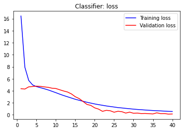
Let’s evaluate the validation and testing accuracies of the model.

让我们评估模型的验证和测试准确性。

val_gen.reset()loss_v, accuracy_v = model.evaluate(val_gen, steps=(val_gen.n / batch_size) + 1, verbose=1)loss, accuracy = model.evaluate(test_gen, steps=(test_gen.n / batch_size) + 1, verbose=1)print("[INFO] Validation: accuracy = %f  ;  loss_v = %f" % (accuracy_v, loss_v))print("[INFO] Test: accuracy = %f  ;  loss_v = %f" % (accuracy, loss))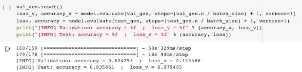

Validation and Test Accuracy Evaluation — Classifier Model

验证和测试准确性评估—分类器模型

This resulted in my classifier model achieving 82.43% validation accuracy and 83.6% testing accuracy. We can push this further by performing some fine-tuning. In the meantime, let’s run up the confusion matrix to visually see how accurate our model is at classifying the produce as of now.

这使我的分类器模型达到了82.43％的验证准确度和83.6％的测试准确度。 通过执行一些微调，我们可以进一步推动这一点。 同时，让我们运行混淆矩阵以直观地看到我们的模型到目前为止对产品进行分类的准确性。

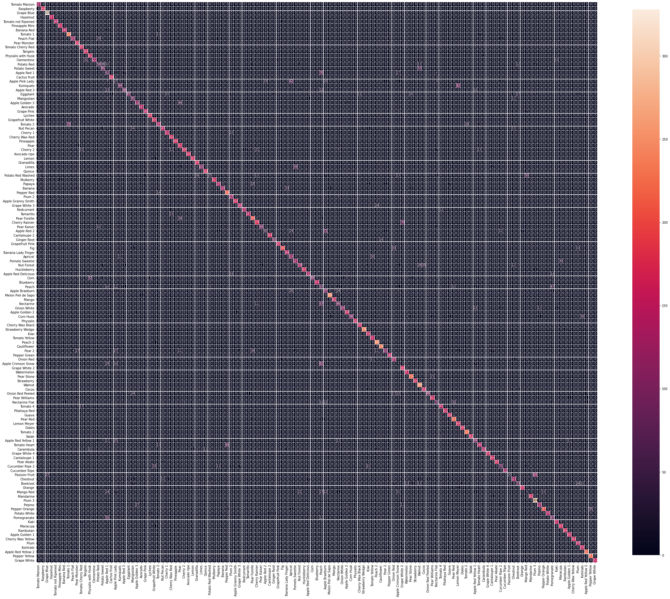
#running predictionsprint('[INFO] running predictions for classifier model...\n')y_pred = model.predict(test_gen, steps=(test_gen.n // batch_size) + 1, verbose=1)y_true = test_gen.classes[test_gen.index_array]plot_confusion_matrix(y_true, y_pred.argmax(axis=-1), labels, out_path=(output_dir+ "/base_confusion_matrix.png"))class_report = classification_report(y_true, y_pred.argmax(axis=-1), target_names=labels)

As you can see, even we though we achieved around 80% accuracy, there are multiple instances where the model seems to misclassify different types of produce, which can be seen by the coloured cells outside the straight coloured line in the image below. Let’s keep working to improve this further.

如您所见，即使我们实现了约80％的准确度，但在很多情况下，该模型似乎仍对不同类型的产品进行了错误分类，可以通过下图的直线上的彩色单元格看到。 让我们继续努力进一步改善这一点。

For now, store the classifier weights. We will make use of them soon.

现在，存储分类器权重。 我们将尽快使用它们。

print('[INFO] locating output directory...')BASE_PATH = os.path.sep.join(["output_files", "base_weights.h5"])print('[INFO] classifier weights have been stored!')model.save(BASE_PATH)

初始化微调模型 (Initialising fine-tuned model)

We will be initialising the same model with a different name, which will hold the pre-trained base’s weights and the weights of our newly trained classifier! This would allow us to pass on the knowledge from the classifier model to this target model.

我们将使用不同的名称来初始化相同的模型，该模型将保留预先训练的基准的权重和我们新训练的分类器的权重！ 这将使我们能够将知识从分类器模型传递到该目标模型。

# FT modeltop_model= models.Sequential()top_model.add(conv_base)top_model.add(layers.Dropout(0.4))top_model.add(layers.Flatten())  # this converts our 3D feature maps to 1D feature vectorstop_model.add(layers.Dense(256, activation='relu', name='fc_1'))top_model.add(layers.Dense(128, activation='relu', name='fc_2'))top_model.add(layers.Dense(len(labels), activation = "softmax", name='predictions'))print('[INFO] fine-tuned model initialised!')

Load the classifier weights we saved before to the target model.

将之前保存的分类器权重加载到目标模型。

print('[INFO] loading classifier weights...')top_model.load_weights('/content/output_files/base_weights.h5')print('[INFO] classifier weights loaded!')

Now that our classifier weights have been loaded onto the model, let’s do a quick parameter check.

现在，我们的分类器权重已加载到模型上，让我们进行快速参数检查。

# checking the amount of trainable parameter in the frozen modeltop_model.summary()

Let’s unfreeze our base by setting all conv_base layers to be trainable.

让我们通过将所有conv_base层设置为可训练来解冻我们的基础。

# unfreezing baseconv_base.trainable = True

Now, let’s set the final block of layers in the conv_base to be the only trainable layers, and display the status of each layer in the base.

现在，让我们将conv_base的最后一层图层设置为唯一可训练的图层，并显示基础中每个图层的状态。

# reset our data generatorstrain_gen.reset()val_gen.reset()# now that the head FC layers have been trained/initialized,# unfreeze the final block of CONV layers and making them trainablefor layer in conv_base.layers[:10]:layer.trainable = False# loop over the layers in the model and show their trainable statusfor layer in conv_base.layers:print("{}: {}".format(layer, layer.trainable))

Again, let’s perform a quick parameter check.

同样，让我们​​执行快速参数检查。

# checking the amount of trainable parameters in the unfrozen model.top_model.summary()

Compile the fine-tuned model.

编译微调的模型。

# compiling the modelprint("[INFO] recompiling model...")top_model.compile(loss='sparse_categorical_crossentropy',optimizer=opt,metrics=['acc'])

Once the model has been compiled, let’s train the model for a final round! *ding ding ding*

编译模型后，让我们训练模型进行最后一轮！ *叮叮叮*

# training the modelprint("[INFO] training FT model...")start = datetime.datetime.now()history = top_model.fit_generator(train_gen,steps_per_epoch=(len(train_gen.filenames) // batch_size) + 1,epochs=trained_epochs,validation_data=val_gen,validation_steps=(len(val_gen.filenames) // batch_size) + 1,verbose=1)end = datetime.datetime.now()elapsed1 = end-start

可视化微调的模型结果 (Visualising fine-tuned model results)

Now that the model has finished training, let’s plot the performance history of our fine-tuned model.

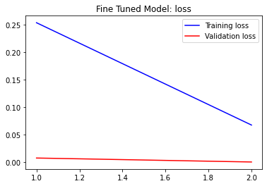
既然模型已经完成训练，那么让我们来绘制经过微调的模型的性能历史。

# plotting performanceacc = history.history['acc']val_acc = history.history['val_acc']loss = history.history['loss']val_loss = history.history['val_loss']epochs = range(1, len(acc) + 1)plt.plot(epochs, acc, 'blue', label='Training acc')plt.plot(epochs, val_acc, 'red', label='Validation acc')plt.title('Fine Tuned Model: accuracy')plt.legend()plt.figure()plt.plot(epochs, loss, 'blue', label='Training loss')plt.plot(epochs, val_loss, 'red', label='Validation loss')plt.title('Fine Tuned Model: loss')plt.legend()plt.show()

These are the results I achieved. You can see that the model achieves around 98% in training accuracy and 94% validation accuracy.

这些是我取得的成果。 您可以看到该模型在训练精度上达到了约98％，在验证精度上达到了94％。

Fine-Tuned Model Accuracy (left), Fine-Tuned Model Loss (right)

精调模型精度(左)，精调模型损失(右)

Let’s evaluate the model on validation and test samples.

让我们在验证和测试样本上评估模型。

val_gen.reset()loss_v, accuracy_v = top_model.evaluate(val_gen, steps=(val_gen.n / batch_size), verbose=1)loss, accuracy = top_model.evaluate(test_gen, steps=(test_gen.n / batch_size), verbose=1)print("[INFO] Validation: accuracy = %f  ;  loss_v = %f" % (accuracy_v, loss_v))print("[INFO] Test: accuracy = %f  ;  loss_v = %f" % (accuracy, loss))

Validation and Test Accuracy Evaluation — Fine-tuned Model

验证和测试准确性评估—精调模型

This resulted in my fine-tuned model achieving 94.09% validation accuracy and 94.87% testing accuracy! Let’s run the confusion matrix up again to visually see how our model’s learning has improved from the previous round.

这使我经过微调的模型达到了94.09％的验证准确度和94.87％的测试准确度！ 让我们再次运行混淆矩阵，以直观地看到我们的模型的学习与上一轮相比有何改进。

#running predictionsprint('[INFO] running predictions for final model...\n')y_pred = top_model.predict(test_gen, steps=(test_gen.n // batch_size) + 1, verbose=1)y_true = test_gen.classes[test_gen.index_array]plot_confusion_matrix(y_true, y_pred.argmax(axis=-1), labels, out_path=(output_dir+ "/ft_confusion_matrix.png"))class_report = classification_report(y_true, y_pred.argmax(axis=-1), target_names=labels)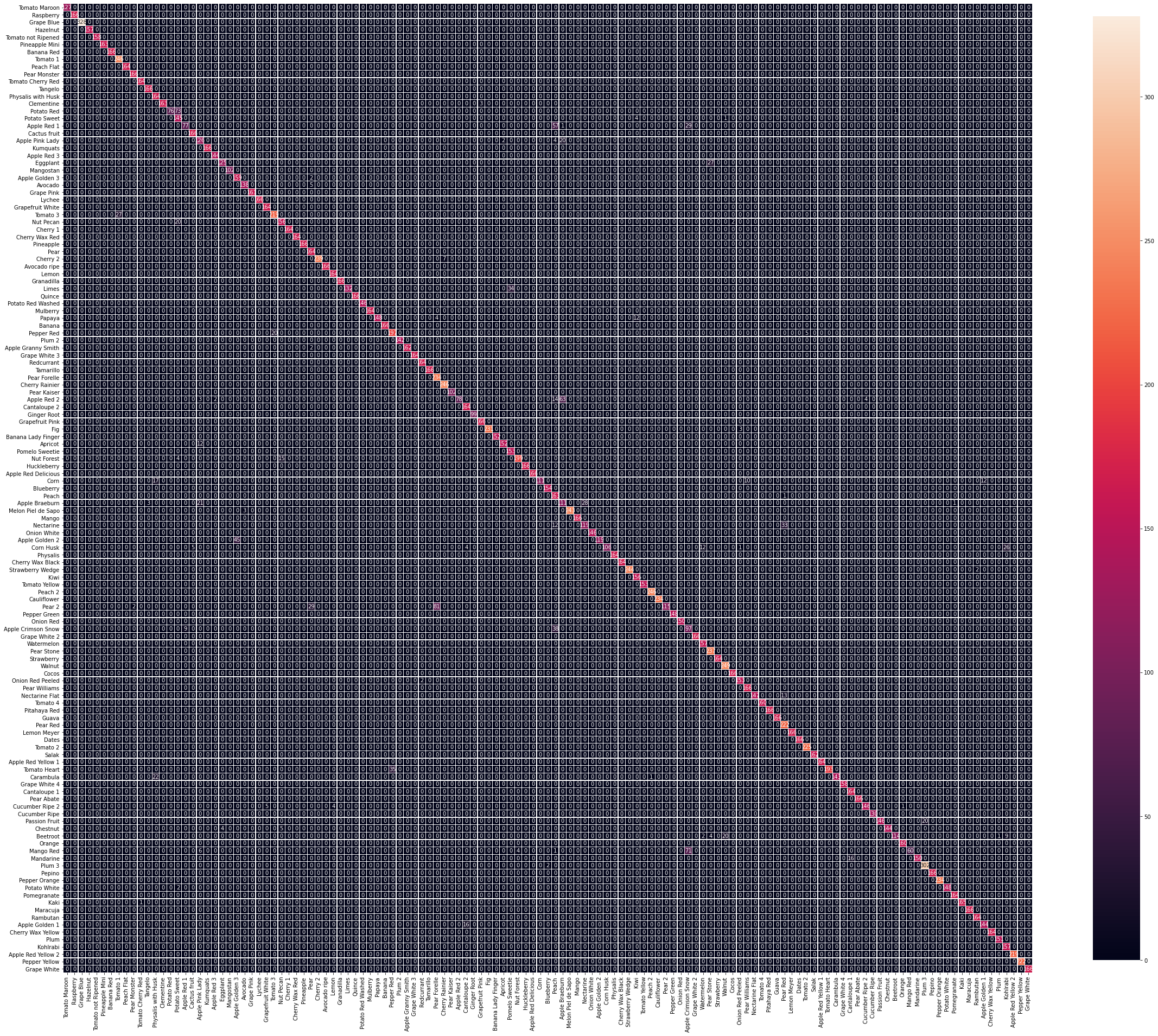

Fine-Tuned Model Confusion Matrix

精调模型混淆矩阵

We can see a significant improvement from the previous confusion matrix, as there are less instances of misclassification compared before. Let’s see the total duration we’ve spent to train the models to achieve these results.

我们可以看到，与以前的混淆矩阵相比，有了很大的改进，因为与以前相比，分类错误的案例更少了。 让我们看看我们训练模型以达到这些结果所花费的总时间。

print('[INFO] Training Model Duration: ', elapsed1)total = elapsed+elapsed1print('[INFO] Total Training Duration: ', total)

We can now store the weights of our final model, which can be used for another project at a later time!

现在，我们可以存储最终模型的权重，该权重可以在以后用于其他项目！

print('[INFO] locating output directory...')TOP_PATH = os.path.sep.join(["output_files", "final_weights.h5"])print('[INFO] final model weights have been stored!')top_model.save(TOP_PATH)

And with that, we have just created our successful image classifier! From freezing the conv_base and performing network surgery to train our custom classifier, to then fine-tuning the model to let it become attuned to the dataset — we have seen the learning accuracy improve, backed by the results we have achieved. We then visualised the results of both training rounds with the help of the figures and confusion matrices to see how accurate the model has gotten from the start of the project. You can save the images of the figures and confusion matrices we plotted earlier, by right-clicking the images and saving them to the image_classifier directory we created at the start.

至此，我们刚刚创建了成功的图像分类器！ 从冻结conv_base到执行网络手术以训练我们的自定义分类器，再到对模型进行微调以使其适应数据集-我们已经看到了学习成果，并提高了学习准确性。 然后，我们借助数字和混淆矩阵将两个训练回合的结果可视化，以查看该模型从项目开始以来的准确性。 通过右键单击图像并将其保存到我们在开始时创建的image_classifier目录中，可以保存我们先前绘制的图形和混淆矩阵的图像。

Future work for this project, would be attempting to add other techniques that would allow the model to classify produce to improve the results we have achieved today.

该项目的未来工作将尝试添加其他技术，以使模型对农产品进行分类，以改善我们今天所取得的成果。

I welcome feedback and constructive criticism as I’m still learning about AI techniques :)

我仍在学习AI技术，欢迎反馈和建设性的批评:)

Link to the notebook repo on my GitHub.

链接到我的GitHub上的笔记本仓库。

Thank you for reading!

感谢您的阅读！

翻译自: https://medium.com/@enrictrillo/an-image-classifier-with-keras-2f0e9b868a36