


pytorch实现梯度下降
介绍 (Introduction)
In machine learning, usually, there is a loss function (or cost function) that we need to find the minimal value. Gradient Descent is one of the optimization methods that is widely applied to do the job.
在机器学习中,通常需要一个损失函数(或成本函数)来寻找最小值。 梯度下降是一种广泛用于完成工作的优化方法之一。
In this post, I will discuss the gradient descent method with some examples including linear regression using PyTorch.
在这篇文章中,我将讨论一些例子,包括使用PyTorch进行线性回归的梯度下降方法。
结石 (Calculus)
One method to find a function’s max or min, it to find the point(s) where the slope equals zero. The max or min of the function will be the solution of the derivative of a function equals zero.
找到函数的最大值或最小值的一种方法是找到斜率等于零的点。 函数的最大值或最小值将是函数导数等于零的解。
Take this function as an example:
以该功能为例:

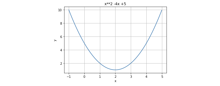
the derivative of the function is:
该函数的派生为:

so let f’(x) = 0, we can find x=2 as the solution. This means the slope of the function equals zero at x=2, and the minimal value of the function is f(2)=1.
因此,令f'(x)= 0,我们可以找到x = 2作为解。 这意味着函数的斜率在x = 2时等于零,函数的最小值为f(2)= 1。
This method finds the analytical solution, however, it is sometimes difficult to apply this method to complex functions in real applications. Therefore, we need numerical methods to find the approximate solution, gradient descent is one of the methods.
该方法找到了解析解,但是,有时很难将此方法应用于实际应用中的复杂功能。 因此,我们需要数值方法来寻找近似解,梯度下降是其中一种方法。
梯度下降 (Gradient Descent)
The mathematical explanation of the gradient can be found in this link.
可以在此链接中找到有关梯度的数学解释。
For one dimension function f(x), the gradient is represented as f’(x). For the multi-dimension function, it is represented as below.
对于一维函数f(x),梯度表示为f'(x)。 对于多维功能,其表示如下。

From wiki: If the gradient of a function is non-zero at a point p, the direction of the gradient is the direction in which the function increases most quickly from p, and the magnitude of the gradient is the rate of increase in that direction.
来自wiki :如果函数的梯度在点p处不为零,则梯度的方向是函数从p开始最快增加的方向,并且梯度的大小是该方向上的增长率。
The gradient descent tries to approach the min value of the function by descending to the opposite direction of the gradient.
梯度下降尝试通过下降到梯度的相反方向来接近函数的最小值。
It updates the parameters (here, x) iteratively to find the solution. So first, we need an initial guess (x0) of the solution, then calculate the gradient based on the initial guess, then based on the calculated gradient to update the solution (x). It can be explained in this formula:
它迭代更新参数(此处为x)以找到解决方案。 因此,首先,我们需要解的初始猜测(x0),然后根据初始猜测计算梯度,然后根据计算出的梯度来更新解(x)。 可以用以下公式解释:

t is the iteration and r is the learning rate.
t是迭代,r是学习率。
So, first, we have an initial guess x0, by the equation above, we can find the x1:
因此,首先,我们有一个初始猜测x0,通过上面的等式,我们可以找到x1:

then by x1, we can find x2:
然后通过x1,我们可以找到x2:

by repeating this process several times (epoch), we should be able to find the parameters (x) where the function at its min value.
通过多次重复此过程(时期),我们应该能够找到函数的最小值处的参数(x)。
范例1: (Example 1:)
Let’s take the previous function as an example:
让我们以先前的功能为例:
and apply it to the gradient descent equation
并将其应用于梯度下降方程
rearrange:
改编:

Let’s set the learning rate = 0.1 and initial guess x0=7. We can then easily update and calculate the x1, x2, x3… and f(x1), f(x2), f(x3)…
让我们将学习率设置为0.1,初始猜测值x0 = 7。 然后,我们可以轻松地更新和计算x1,x2,x3…和f(x1),f(x2),f(x3)…
In this example:
在此示例中:
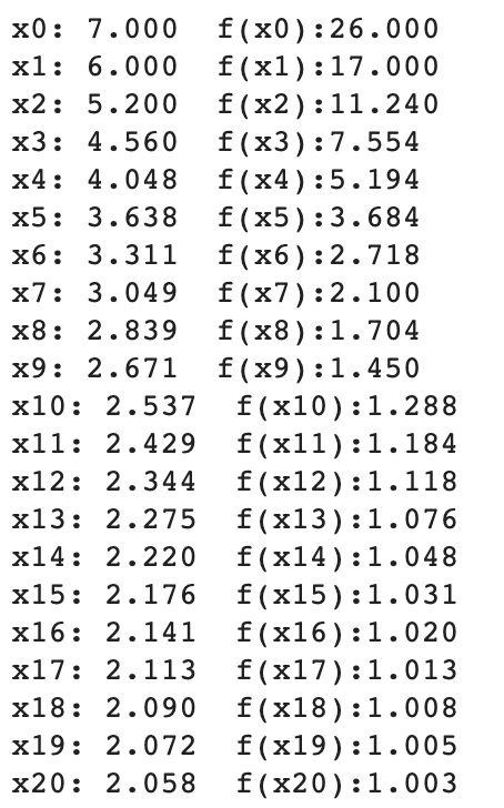
You can see the parameter (x) approaches to 2 and the function approaches its min value 1.
您可以看到参数(x)接近2,函数接近其最小值1。
Let’s put it on the graph:
让我们把它放在图表上:
What if we use a smaller learning rate (0.01)?
如果我们使用较小的学习率(0.01)怎么办?
As expected, it took more iterations to reach the minimum.
如预期的那样,需要更多的迭代才能达到最小值。
If we increase the learning to 0.3, it reached the minimum faster than 0.1.
如果我们将学习增加到0.3,则达到最小值的速度快于0.1。
If we increase it further to 0.7, it started to overshoot.
如果将其进一步增加到0.7,它就会开始超调。

If we increase it to 1, it cannot reach the minimum value at all.
如果将其增加到1,则根本无法达到最小值。
So the learning rate is very important to gradient descent. If it is too small, a lot of iterations are needed, if it is too big, it might not be able to reach the minimum.
因此,学习率对于梯度下降非常重要。 如果值太小,则需要大量迭代;如果值太大,则可能无法达到最小值。
Now, we have an idea of how the gradient descent work, let’s try to apply that to a simple machine learning model — linear regression.
现在,我们对梯度下降的工作原理有所了解,让我们尝试将其应用于简单的机器学习模型-线性回归。
示例2 —线性回归: (Example 2 — linear regression:)
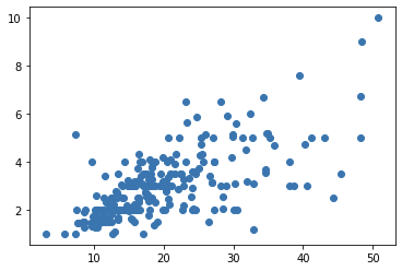
Linear regression is an approach to find a linear relationship between two variables. It finds a line,
线性回归是一种在两个变量之间寻找线性关系的方法。 找到一条线,

that describes the data points shown in the figure. m is the slope of the line and c is the intercept. The task is to find the line (m and c) that best fits the data points.
描述了图中所示的数据点。 m是直线的斜率,c是截距。 任务是找到最适合数据点的线(m和c)。
Loss function
损失函数
We use Mean Squared Error (MSE) to measure the error of the line and data points.
我们使用均方误差(MSE)来测量线和数据点的误差。

It averages the square of the sum of the differences between points and the line.
它平均点与线之间的差之和的平方。
We can rearrange the equation:
我们可以重新排列等式:

We want to find the m and c, which gives the minimum value of MSE.
我们想要找到m和c,它们给出了MSE的最小值。
Gradient Descent
梯度下降
Just like the previous example, we need to find the gradient.
就像前面的示例一样,我们需要找到渐变。

Then we can use this equation to update m and c:
然后我们可以使用以下等式更新m和c:

Again, we need an initial guess for m and c, let’s start with m=0 and c=0, with learning rate = 0.0001
同样,我们需要对m和c进行初步猜测,让我们从m = 0和c = 0开始,学习率= 0.0001
#Gradient Descentfor i in range(epochs):
   Y_pred = m*X + c
   d_m = (-2/n) * sum(X * (Y - Y_pred))
   d_c = (-2/n) * sum(Y - Y_pred)
   # Update m
   m = m - r * d_m
   # Update c
   c = c - r * d_c
   mse=(1/n) * sum((Y - m*X + c)**2)
The m and c can be updated based on the gradient. Let’s put it on the graph.
可以基于梯度更新m和c。 让我们把它放在图表上。
Again, a carefully chosen learning rate is important, if the learning rate is increased to 0.01, the calculation will not converge.
同样,精心选择的学习速率很重要,如果将学习速率提高到0.01,则计算将不会收敛。
In this simple example, we are calculating the gradient by taking the derivative of the function ourselves, it might become difficult for a more complicated problem. Luckily, PyTorch provides a tool to automatically compute the derivative of nearly any function.
在这个简单的示例中,我们通过自己求函数的导数来计算梯度,对于更复杂的问题可能会变得困难。 幸运的是,PyTorch提供了一种工具,可以自动计算几乎所有函数的导数。
Pytorch approach
火炬方法
Let’s define the line:
让我们定义这一行:
def f(x, params):
    m, c= paramsreturn m*x + c
and the loss function — Mean Squared Error:
和损失函数—均方误差:
def mse(preds, targets): return ((preds-targets)**2).mean()Again, we start by m=0, c=0, the requires_grad_(), is used here to calculate the gradient.
同样,我们从m = 0,c = 0开始, required_grad_()在这里用于计算梯度。
params = torch.zeros(2).requires_grad_()Then we can predict the y values based on our first parameter, and plot it.
然后,我们可以根据第一个参数预测y值,并将其绘制出来。
preds = f(X_t, params)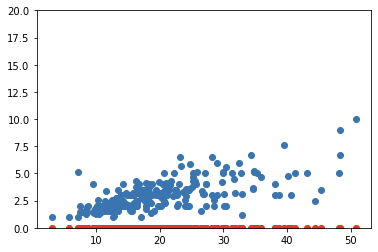
Then we can calculate the loss:
然后我们可以计算损失:
loss = mse(preds, Y_t)and the gradient by this PyTorch function:
以及此PyTorch函数的渐变:
loss.backward()after this we can check the gradient:
之后,我们可以检查渐变:
params.gradit returns a tensor, which is the gradient: tensor([433.6485, 18.2594])
它返回一个张量,即梯度:张量([433.6485,18.2594])
Then we update the parameter using the gradient and learning rate:
然后,我们使用梯度和学习率更新参数:
lr = 1e-4
params.data -= lr * params.grad.data
params.grad = None
and predict the y using these new parameters:
并使用以下新参数预测y:
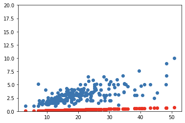
We need to repeat this process several times, let’s make a function:
我们需要重复此过程几次,让我们创建一个函数:
def apply_step(params):
preds = f(X_t, params)
loss = mse(preds, Y_t)
loss.backward()
params.data -= lr * params.grad.data
params.grad = None
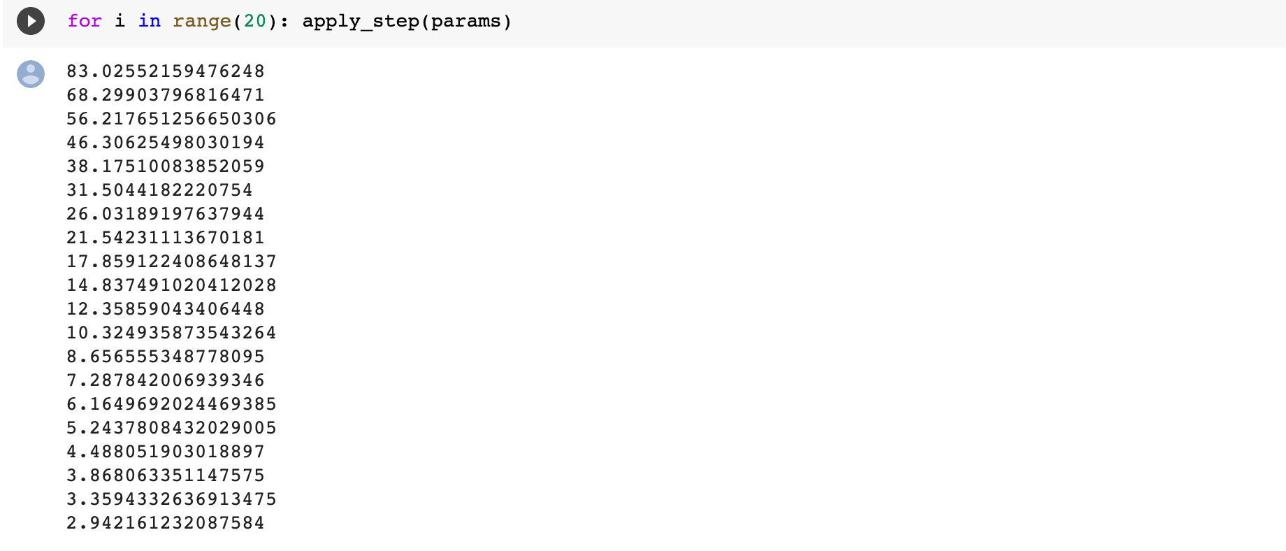
return predThen we can run for several epochs. Looks like the loss is decreasing through epochs.
然后,我们可以运行几个时代。 看起来损失正在减少。
Put it on a graph
放在图上
This is it! By using PyTorch, we can easily calculate the gradient and perform the gradient descent for machine and deep learning models.
就是这个! 通过使用PyTorch,我们可以轻松计算梯度并针对机器和深度学习模型执行梯度下降。
Thanks for reading.
谢谢阅读。
pytorch实现梯度下降


 1579
1579


 被折叠的 条评论
为什么被折叠?
被折叠的 条评论
为什么被折叠?
 到【灌水乐园】发言


