回归分析法_回归分析

回归分析法

In Supervised Learning, we mostly deal with two types of variables i.e numerical variables and categorical variables. Wherein regression deals with numerical variables and classification deals with categorical variables. Where,

在监督学习中，我们主要处理两种类型的变量，即数值变量和分类变量。 其中， 回归处理数字变量， 分类处理类别变量。 哪里，

Regression is one of the most popular statistical techniques used for Predictive Modelling and Data Mining in the world of Data Science. Basically,

回归 是数据科学领域中用于预测建模和数据挖掘的最受欢迎的统计技术之一。 基本上，

Regression Analysis is a technique used for determining the relationship between two or more variables of interest.

回归分析是一种用于确定两个或多个目标变量之间的关系的技术。

However, Generally only 2–3 types of total 10+ types of regressions are used in practice. Linear Regression and Logistic Regression being widely used in general. So, Today we’re going to explore following 4 types of Regression Analysis techniques:

但是，在实践中，通常总共使用10种以上的回归类型中只有2–3种类型。 线性回归和逻辑回归通常被广泛使用。 因此，今天我们将探讨以下4种类型的回归分析技术：

• Simple Linear Regression

  简单线性回归

• Ridge Regression

  岭回归

• Lasso Regression

  套索回归

• ElasticNet Regression

  ElasticNet回归

We will be observing their applications as well as the difference among them on the go while working on Student’s Score Prediction dataset. Let’s get started.

在研究学生的分数预测数据集时，我们将随时随地观察它们的应用以及它们之间的差异。 让我们开始吧。

1.线性回归 (1. Linear Regression)

It is the simplest form of regression. As the name suggests, if the variables of interest share a linear relationship, then Linear Regression algorithm is applicable to them. If there is a single independent variable(here, Hours), then it is a Simple Linear Regression. If there are more than 1 independent variables, then it is a Multiple Linear Regression. The mathematical equation that approximates linear relationship between independent (criterion ) variable X and dependent(predictor) variable Y is:

这是回归的最简单形式。 顾名思义，如果感兴趣的变量具有线性关系，则线性回归算法适用于它们。 如果只有一个自变量(此处为Hours)，则为简单线性回归 。 如果有超过1个自变量，则为多元线性回归 。 近似自变量(标准)X和因变量(预测变量)Y之间的线性关系的数学公式为：

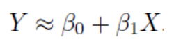
where, β0 and β1 are intercept and slope respectively which are also known as parameters or model co-efficients.

其中，β0和β1分别是截距和斜率，也称为参数或模型系数。

Regression analysis is used to find equations that fit data. Once we have the regression equation(the one as above to observe correlation between X and Y), we can use the model to make predictions. When a correlation coefficient shows that data is likely to be able to predict future outcomes and a scatter plot of the data appears to form a straight line , you can use simple linear regression to find a predictive function. Let’s try this out, shall we?

回归分析用于查找适合数据的方程式。 一旦有了回归方程(上面的那个用来观察X和Y之间的相关性)，就可以使用该模型进行预测。 当一个 相关系数表明数据很可能能够预测将来的结果，并且数据的散点图似乎形成一条直线，您可以使用简单的线性回归来找到预测函数。 让我们尝试一下，好吗？

数据集概述 (Overview of Dataset)

Since we are focusing on regression analysis, I have chosen relatively small dataset. Hence, we won’t be needing the Data Wrangling part.

由于我们专注于回归分析，因此我选择了相对较小的数据集。 因此，我们将不需要数据整理部分。

可视化数据分布 (Visualizing Data Distribution)

From the above plots, We can see that the distribution of data is a little skewed. We can say this because we observe the data distribution here with the classic ‘bell-shaped’ data distribution curve as a reference.

从上面的图中可以看出，数据的分布有些偏斜。 之所以说是因为我们在这里观察到的数据分布以经典的“钟形”数据分布曲线为参考。

可视化变量之间的关系 (Visualizing Relationship Between Variables)

In the above plot, we can see that the relationship between Hours and Scores is linear. The green points are the actual observations while the green line is the best fit line of regression. This shall give us a strong positive correlation between Scores and Hours (since the slope of the line is increasing in the positive direction). Let’s verify.

在上图中，我们可以看到小时和分数之间的关系是线性的。 绿点是实际观察值，而绿线是回归的最佳拟合线。 这将使我们在分数和小时数之间具有很强的正相关性(因为直线的斜率沿正方向增加)。 让我们验证一下。

Visualizing Degree of Correlation Between Variables

可视化变量之间的相关程度

Clearly, scores and hours have very strong correlation coefficient i.e 0.98. Now, let’s apply and explore our regression algorithms.

显然，分数和小时数具有非常强的相关系数，即0.98。 现在，让我们应用和探索我们的回归算法。

First of all, Let’s fit our data to the Linear Regression model and check out how the accuracy of the model turns out.

首先，让我们将数据拟合到线性回归模型，并检查模型的准确性。

Now, let’s check out the performance of other models.

现在，让我们检查一下其他模型的性能。

2.岭回归 (2. Ridge Regression)

The Ridge regression is again a statistical technique which is used to analyze multiple regression data which is multicollinear in nature or when the number of predictor(dependent) variables are more than the number of criterion(independent) variables. The concept of multicollinearity occurs when correlation occurs among two or more predictor(dependent) variables.

Ridge回归还是一种统计技术，用于分析本质上是多重共线性的或当预测变量(因变量)的数量大于标准变量(因变量)的数量时的多元回归数据。 当两个或多个预测变量(因变量)之间发生相关时，就会出现多重共线性的概念。

Ridge regression performs L2 Regularization technique.

Ridge回归执行L2正则化技术。

A regularization technique is a technique used to:

正则化技术是用于以下目的的技术：

• Minimize the error between estimated and actual values/observations
  最小化估计值与实际值/观测值之间的误差
• To reduce(regularize) the magnitude of the co-efficients of features/parameters or ultimately the cost function per se.
  减少(正则化)特征/参数系数的大小或最终降低成本函数本身。

As ridge regression shrinks(regularizes/reduces) the co-efficients of parameters of it’s equation(as shown in the snippet below) towards zero, it introduces some bias. But it can reduce the variance to a great extent which will result in a better mean-squared error i.e increasing the accuracy. The amount of shrinkage is controlled by parameter λ which multiplies the ridge penalty(i.e introduces bias). Higher the λ, Higher the shrinkage. Thus,we can get different coefficient estimates for the different values of λ.

岭回归 将其方程式参数的系数(如下面的代码片段所示)缩小(正则化/缩小)为零，这会引入一些偏差。 但是它可以在很大程度上减小方差，这将导致更好的均方误差，即提高精度 。 收缩量受参数λ的控制，该参数乘以脊线损失 (即引入偏差)。 λ越高，收缩率越高。 因此，对于不同的λ值，我们可以获得不同的系数估计。

Cost Function of Ridge regression can be mathemattically represented as:

Ridge回归的成本函数可以用数学表示为：

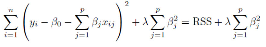
where, RSS=Residual Sum of Squares which is nothing but the sum of square of deviation between actual values and the values predicted by the model.

其中，RSS =残差平方和，仅是实际值与模型预测的值之间的偏差平方和。

For finding λ, cross-validation technique is used. So, Let’s find the best estimate of λ for our dataset and see how the accuracy turns out.

为了找到λ，使用交叉验证技术。 因此，让我们为我们的数据集找到最佳的λ估计值，然后看看结果如何。

Here, RidgeCV has built-in cross-validation for ridge regression algorithm which is used to find the best estimate for our λ parameter(here, known as alpha). Hence, we define a list alphas consisting lowest to highest range of values. Then, we pass this list as a parameter in RidgeCV and find out our best estimate. We got alpha=0.01155 for our dataset. Then, we pass this alpha as a paremeter in our Ridge regression model and evaluate it’s accuracy.

在这里，RidgeCV具有针对岭回归算法的内置交叉验证，该算法用于找到我们的λ参数(此处称为alpha)的最佳估计。 因此，我们定义了一个列表Alpha，该列表的Alpha值范围从最低到最高。 然后，我们将此列表作为RidgeCV中的参数传递，并找出我们的最佳估计。 我们的数据集的alpha = 0.01155。 然后，我们将此alpha用作我们的Ridge回归模型中的参数，并评估其准确性。

This surely optimized our Mean Absolute Error from 4.18 to 4.05 and Root Mean Squared Error from 4.65 to 4.56.

这无疑将我们的平均绝对误差从4.18最佳化为4.05，将均方根误差从4.65最佳化至4.56。

3.套索回归 (3. Lasso Regression)

The acronym ‘LASSO’ stands for Least Absolute Shrinkage and Selection Operator. As the name indicates, this algorithm can perform in-built variable(feature) selection as well as parameter shrinkage. Shrinkage is where data values are shrunk towards a central point, like the mean.

缩写“套索”代表对于L 东 bsolute 小号 hrinkage和S选操作结束时切。 顾名思义，该算法可以执行内置变量(功能)选择以及参数缩小。 收缩是数据值向中心点(如均值) 收缩的地方。

So, Lasso Regression uses L1 Regularization technique. The objective function of Lasso Regression is:

因此，套索回归使用L1正则化技术。 拉索回归的目标函数是：

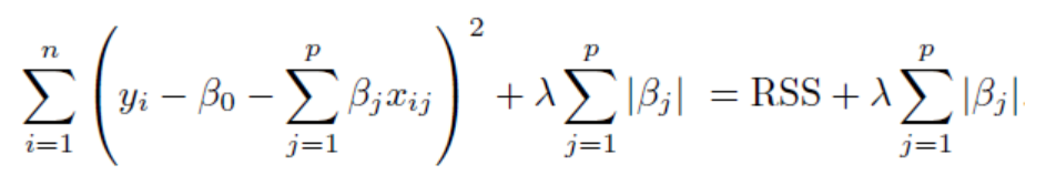
where, RSS= Residual Sum of Squares and λ is the shrinkage parameter.

其中，RSS =残差平方和，而λ是收缩参数。

The difference between Ridge & Lasso regression is as follows:

Ridge＆Lasso回归之间的差异如下：

• Cost function of Lasso regression also contains shrinkage parameter but unlike Ridge regression, the estimated co-efficient βj’s absolute value is considered and not squared.
  Lasso回归的成本函数也包含收缩参数，但是与Ridge回归不同，估计系数βj的绝对值是考虑的而不是平方的。
• In Ridge regression, the shrinkage parameter regularizes the value of estimated co-efficient to tend to zero but not absolute zero. Whereas, in Lasso regression, it can make the estimated co-efficient absolute zero in accordance with the feature selection.
  在Ridge回归中，收缩参数将估计系数的值调整为趋于零而不是绝对零的趋势。 而在套索回归中，可以根据特征选择使估计系数的绝对值为零。

The ability of Lasso regression mentioned in the second point thus makes it easier to interpret.

第二点提到的套索回归的能力因此使其更易于解释。

Now, Let’s implement a Lasso regression model and observe how the accuracy of the predictions turns out.

现在，让我们实现一个套索回归模型，并观察预测的准确性如何。

Here, the LassoCV library is used for estimating the best value for λ paremeter(also known as alpha as shown in the parameters in the below code snippet). We have used 10-fold cross-validation for finding our best estimate. Now, let’s look at the evaluation metrics.

在这里，LassoCV库用于估计λ参数的最佳值(也称为alpha，如下面的代码片段中的参数所示)。 我们使用10倍交叉验证来找到最佳估计值。 现在，让我们看一下评估指标。

The Mean Absolute Error has been reduced to 4.03 from 4.05 and The Root Mean Squared Error has been reduced to 4.55 from 4.56. Note that both Lasso & Ridge optimized the evaluation metrics more effectively than the Simple Linear Regression.

平均绝对误差已从4.05降低至4.03，均方根误差已从4.56降低至4.55。 请注意，套索和里奇均比简单线性回归更有效地优化了评估指标。

4. ElasticNet回归 (4. ElasticNet Regression)

• ElasticNet Regression uses both L1 and L2 Regularization techniques.
  ElasticNet回归同时使用L1和L2正则化技术。
• It can perform feature selection and regularization(shrinking the parameters) simultaneously.
  它可以同时执行特征选择和正则化(缩小参数)。
• ElasticNet model can select ’n’ number of features until saturation whereas Lasso model tends to choose one feature from various correlated groups of features.
  ElasticNet模型可以选择'n'个特征，直到饱和为止，而Lasso模型倾向于从各种相关的特征组中选择一个特征。

Hence, we can say that it draws the advantages of both the worlds i.e Lasso & Ridge regressions. ElasticNet regression can be mathematically represented as:

因此，可以说，它利用了两个世界的优势，即Lasso＆Ridge回归。 ElasticNet回归可以用数学表示为：

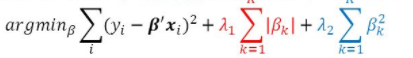
where, λ1 and λ2 are L1 & L2 norms respectively. We can clearly see in the equation that cost function of ElasticNet regression consists of estimated co-efficients from both Lasso and Ridge regressions alongwith the first term as RSS.

其中，λ1和λ2分别是L1和L2范数。 我们可以从方程式中清楚地看到，ElasticNet回归的成本函数由来自Lasso和Ridge回归以及第一项作为RSS的估计系数组成。

Here, we use GridSearchCV to perform 10-fold cross-validation and pass a list of smallest to largest possible values of alpha in the alpha parameter so that it gives us the best estimate for alpha. Now, let’s implement the ElasticNet model and check how the evaluation metrics turns out.

在这里，我们使用GridSearchCV进行10倍交叉验证，并在alpha参数中传递最小到最大的alpha值列表，以便为我们提供最佳的alpha估计。 现在，让我们实现ElasticNet模型，并检查评估指标的结果。

The Mean Absolute Error reduced from 4.03 to 3.94 and the Root Mean Squared Error reduced from 4.55 to 4.5.

平均绝对误差从4.03降低到3.94，均方根误差从4.55降低到4.5。

Thus, we can optimize a Regression problem’s performance.

因此，我们可以优化回归问题的性能。

谢谢！ (Thank You!)

翻译自: https://medium.com/swlh/revisiting-regression-analysis-2ff050fb8b89

回归分析法