使用python arima第2部分1创建预测

最新推荐文章于 2023-02-05 16:29:32 发布

weixin_26729165

最新推荐文章于 2023-02-05 16:29:32 发布

阅读量1k

点赞数

文章标签： python java

原文链接：https://medium.com/swlh/create-forecast-using-python-arima-part-2-1-efca5c5c14f3

版权

This tutorial was created to democratize data science for business users (i.e., minimize usage of advanced mathematics topics) and alleviate personal frustration we have experienced on following tutorials and struggling to apply that same tutorial for our needs. Considering this, our mission is as follows:

创建本教程的目的是使业务用户的数据科学民主化(即，最大限度地减少高级数学主题的使用)，并减轻我们在后续教程中遇到的个人挫败感，并努力将同一教程应用于我们的需求。 考虑到这一点，我们的任务如下：

Provide practical application of data science tasks with minimal usage of advanced mathematical topics
以最少的高级数学主题提供数据科学任务的实际应用
Only use a full set of data, which are similar to data we see in business environment and that are publicly available in a tutorial, instead of using simple data or snippets of data used by many tutorials
仅使用与我们在业务环境中看到的数据相似并且在教程中公开可用的全套数据，而不是使用简单数据或许多教程使用的数据片段
Clearly state the prerequisites at beginning of the tutorial. We will try to provide additional information on those prerequisites
在教程开始时清楚地说明先决条件。 我们将尝试提供有关这些先决条件的其他信息
Provide written tutorial on each topic to ensure all steps are easy to follow and clearly illustrated
提供有关每个主题的书面教程，以确保所有步骤都易于遵循并清楚地说明

1.说明(1. Description)

This is multi-part series on how to create a forecast, using one of the most widely used data science tool — Python.

这是有关如何使用最广泛使用的数据科学工具之一Python创建预报的多部分系列文章。

Forecasting is the process of making predictions of the future based on past and present data and its trends. The accuracy of forecast decreases as you stretch out your forecast. For example, if you are forecasting monthly sales then accuracy of forecast for month 1 sales of forecast will be higher than month 2 sales of forecast and so on. One of my co-workers likes to state that best way to predict tomorrow’s weather is to assume it is similar to today’s weather. Everything else is just a guess.

预测是根据过去和现在的数据及其趋势对未来进行预测的过程。延伸预测时，预测的准确性会降低。例如，如果您正在预测月度销售，则预测的第一个月的销售的预测准确性将高于预测的第二个月的销售，依此类推。我的一位同事喜欢说，预测明天天气的最好方法是假设它与今天的天气相似。其他所有只是猜测。

Forecasting Series consists of:

预测系列包括：

Part 1.1 — Create Forecast using Excel 2016/2019 (https://medium.com/@sungkim11/data-science-for-business-users-f4c050cbec96)
第1.1部分-使用Excel 2016/2019创建预测( https://medium.com/@sungkim11/data-science-for-business-users-f4c050cbec96 )
Part 1.2 — Fine-Tune Forecast using Excel 2016/2019
第1.2部分—使用Excel 2016/2019进行微调预测
Part 2.1 — Create Forecast using Python — ARIMA
第2.1部分-使用Python创建预测-ARIMA
Part 2.2 — Advanced Topics on Forecast using Python — ARIMA
第2.2部分-使用Python进行预测的高级主题-ARIMA
Part 2.3 — Extend Forecast (Python) to include What-If Analysis Capabilities — ARIMA
第2.3部分-扩展预测(Python)以包括假设分析功能-ARIMA
Part 3.1 — Create Forecast using Python — Prophet (https://medium.com/@sungkim11/create-forecast-using-python-prophet-3-1-5ea64c3b103b)
第3.1部分-使用Python创建预测-先知( https://medium.com/@sungkim11/create-forecast-using-python-prophet-3-1-5ea64c3b103b )
Part 3.2 — Advanced Topics on Forecast using Python — Prophet
第3.2部分-使用Python进行预测的高级主题-Prophet
Part 3.3 — Extend Forecast (Python) to include What-If Analysis Capabilities — Prophet
第3.3部分-扩展预测(Python)以包括假设分析功能-先知
Part 4.1 — Create Forecast using Python — LSTM (https://medium.com/@sungkim11/create-forecast-using-python-lstm-4-1-1ab8b138a08f)
第4.1部分-使用Python创建预测-LSTM( https://medium.com/@sungkim11/create-forecast-using-python-lstm-4-1-1ab8b138a08f )
Part 4.2 — Advanced Topics on Forecast using Python — LSTM
第4.2部分—使用Python进行预测的高级主题— LSTM
Part 4.3 — Extend Forecast (Python) to include What-If Analysis Capabilities — LSTM
第4.3部分—扩展预测(Python)以包括假设分析功能— LSTM

2.先决条件 (2. Prerequisites)

Following are prerequisite software for this tutorial:

以下是本教程的必备软件：

- [x] Python (Download Anaconda Python from here => https://www.anaconda.com/download/ and install on your computer.)
- [x] Python Package: pmdarima (Install using "pip install pmdarima" in your Anaconda Prompt). All other python packages used in this tutorial comes with Anaconda Python. 

To install pmdarima on Windows, follow these instructions. It seems pmdarima does not like python 3.7 as of January 2019:

* Create a new virtual environment by "conda create -n arima python=3.5"
* When prompted, enter 'y' to proceed
* Activate new virtual environment by "conda activate arima"
* Install pmdarima by "pip install pmdarima"You can also use Google Colab (https://colab.research.google.com/) as we have done for this tutorial.

Following are prerequisite knowledge for this tutorial:

以下是本教程的先决知识：

- [x] Create Forecast Using Excel 2016/2019 tutorial
- [x] Basic knowledge Python (You really do not need to be expert in python to use python for data science tasks. Many data scientists supplement their basic knowledge of python with google :-) to complete their tasks. We will provide a tutorial soon...
- [x] Basic knowledge installing Python packages (Good news is that Anaconda simplifies this for you somewhat, but they only have limited selection of packages you may need - e.g., pmdarima, which is used in this tutorial cannot be installed using this method). We will provide a tutorial soon...
- [x] Basic knowledge Jupyter Notebook/Lab (Good news is that Jupyter Notebook/Lab is easy to use and learn). We will provide a tutorial soon...
- [x] Basic knowledge Pandas (Pandas is data analysis tools for the Python programming language. This is one of the tool where more you know will make your job easier and there is always google :-). We will provide a tutorial soon...
- [x] Basic knowledge statistical data visualization tool, such as matplotlib, seaborn, bokeh, or plotly (These are data visualization tool for the Python programming language. These are a set of the tool where more you know will make your job easier and there is always google :-). We will provide a tutorial soon...
- [x] Historical data with same frequency (e.g., hourly, daily, weekly, monthly, quarterly, yearly, etc.), to create a forecast. This is important since you cannot create a forecast without historical data that does not have same frequency. If your data does not follow same frequency, then aggregate your data so it will be same frequency. For example, if your data consists of any random two days per week then aggregate (i.e., sum up those two days) your data into a weekly data then create a forecast using aggregated data.

3.步骤 (3. Steps)

Please follow the step by step instructions, which is divided into 8 major steps as shown below:

请按照分步说明进行操作，该说明分为8个主要步骤，如下所示：

Get Data
获取数据
Format Data
格式化数据
Import Data
汇入资料
Cleanse Data
清理数据
Analyze Data
分析数据
Prep Data
准备数据
Develop and Validate Forecast Model
开发和验证预测模型
Maintain Forecast
维持预测

3.1。获取数据 (3.1. Get Data)

United Stated Census Bureau maintains Monthly Retail Trade Report, from January 1992 to Present. This data was picked to illustrate forecasting because it has extensive historical data with same monthly frequency. Data is available as Excel spreadsheet format at https://www.census.gov/retail/mrts/www/mrtssales92-present.xls

美国人口普查局维护从1992年1月至今的每月零售贸易报告。选择该数据是为了说明预测，因为它具有每月频率相同的大量历史数据。数据以Excel电子表格格式提供，网址为https://www.census.gov/retail/mrts/www/mrtssales92-present.xls

1. Click on the link to save Excel spreadsheet to your local directory/folder.

1.单击链接以将Excel电子表格保存到本地目录/文件夹。

2. Open the Excel spreadsheet (i.e., Monthly Trade Report).

2.打开Excel电子表格(即每月贸易报告)。

3. Monthly Retail Trade Report is organized by year where each year from 1992 to 2018 are separated by worksheet. Within each worksheet, there are two different types of figures — not adjusted and adjusted. For each type, there is summary set of figures followed by more detailed figure, organized by NAICS Code (i.e., North American Industry Classification System — the standard used by Federal statistical agencies in classifying business establishments for the purpose of collecting, analyzing, and publishing statistical data related to the U.S. business economy.).

3.月度零售贸易报告按年份组织，其中1992年至2018年之间每年均按工作表分开。在每个工作表中，有两种不同类型的数字-未调整和已调整。对于每种类型，都有一组摘要图，然后是更详细的图，这些图由NAICS代码组织(即北美行业分类系统，这是联邦统计机构用于对企业进行分类以收集，分析和发布的标准)与美国商业经济有关的统计数据。)。

3.2。格式化数据 (3.2. Format Data)

We will need to format the data in Monthly Trade Report, so we can create a forecast from consolidated multiple years of data. At the same time, this data is bit more extensive then we would like, so we will be filtering data as follow:

我们将需要在“每月贸易报告”中格式化数据，以便我们可以根据合并的多年数据创建预测。同时，此数据比我们想要的要广泛得多，因此我们将按以下方式过滤数据：

Use January 2005 to Present time to ensure cyclic behavior (full economic cycle with boom and recession) is represented in our data
使用2005年1月来表示时间，以确保周期性行为(充满景气和衰退的整个经济周期)体现在我们的数据中
Use “NOT ADJUSTED” data as illustrated on cell line 7 to line 12 on the spreadsheet. Other data is nice, but it is bit much for our needs
使用电子表格上第7行到第12行中所示的“ NOT ADJUSTED”数据。其他数据很好，但是可以满足我们的需求

1. Insert a new worksheet, entitled “Forecast”.

1.插入一个新的工作表，标题为“ Forecast”。

2. Copy and paste data from 2005 worksheet into “Forecast” worksheet. When pasting data, use “Transpose” option on Paste. It is easier to scroll up and down then scroll sideways to see the data.

2.将2005年工作表中的数据复制并粘贴到“预测”工作表中。粘贴数据时，请在“粘贴”上使用“移调”选项。上下滚动然后横向滚动查看数据会更容易。

3. Repeat the step 2 for 2006 thru 2018.

3.重复2006年到2018年的步骤2。

4. Copy and paste column label at top of pasted data. Again when pasting data, use “Transpose” option on paste.

4.复制列标签并将其粘贴在粘贴数据的顶部。再次粘贴数据时，在粘贴上使用“转置”选项。

5. Insert date column at left of pasted data, start with 01/01/2005 on first row then 02/01/2005 on second row then fill the rows with date. The end date should be 10/01/2018.

5.在粘贴数据的左侧插入日期列，从第一行的01/01/2005开始，然后在第二行的02/01/2005开始，然后用日期填充行。结束日期应该是10/01/2018。

6. Save the spreadsheet as mrtssales92-present_step2.xlsx.

6.将电子表格另存为mrtssales92-present_step2.xlsx。

3.3。汇入资料 (3.3. Import Data)

Unlike Excel, which is all in one application, you will need to import data into python — specifically pandas (Python Data Analysis Library), which is python’s in-memory database where you can perform data analysis and modeling.

与Excel完全集成在一个应用程序中不同，您需要将数据导入python-特别是pandas(Python数据分析库)，它是python的内存数据库，您可以在其中执行数据分析和建模。

3.3.1. Export Excel data to CSV file

3.3.1。将Excel数据导出到CSV文件

1. Open Excel worksheet, entitled “mrtssales92-present_step2.xlsx”.

1.打开Excel工作表，标题为“ mrtssales92-present_step2.xlsx”。

2. Navigate to “Forecast” worksheet and convert all numbers to just number — e.g., 330000 instead of 330,000. Since 330000 is imported as number and 330,000 is imported as text. It is easier this way. Otherwise, you will need to programatically change data type.

2.导航到“预测”工作表，然后将所有数字转换为仅数字，例如330000而不是330,000。由于330000作为数字导入，330,000作为文本导入。这样比较容易。否则，您将需要以编程方式更改数据类型。

3. Extend the date that currently ends on 10/1/2018 to 12/1/2020 since we will be creating forecast to December 2020.

3.因为我们将创建预测到2020年12月，所以将当前结束日期从10/1/2018延长到12/1/2020。

4. Save the worksheet as CSV file format, entitled “mrtssales92-present_step3.csv”.

4.将工作表另存为CSV文件格式，标题为“ mrtssales92-present_step3.csv”。

3.3.2. Import Python Packages

3.3.2。导入Python包

Best analogy of Python as programming language is that of smart phone. Python is great programming language where you can accomplish a lot of tasks, just like brand new smart phone. Just like brand new smart phone, it is bit limited since it can only accomplish basic tasks without apps that excels at special tasks, such as Google Map. Python packages are similar to smart phone apps where these packages can accomplish specific tasks very well, such as pandas.

Python作为编程语言的最佳比喻是智能手机。 Python是一种很棒的编程语言，您可以在其中完成许多任务，就像全新的智能手机一样。就像全新的智能手机一样，它也有一定的局限性，因为它只能完成基本任务，而没有能够执行特殊任务的应用程序，例如Google Map。 Python程序包类似于智能手机应用程序，其中这些程序包可以很好地完成特定任务，例如熊猫。

1. Install pmdarima python package

1.安装pmdarima python软件包

!pip install pmdarimaRequirement already satisfied: pmdarima in /usr/local/lib/python3.6/dist-packages (1.7.0)
Requirement already satisfied: statsmodels>=0.11 in /usr/local/lib/python3.6/dist-packages (from pmdarima) (0.11.1)
Requirement already satisfied: joblib>=0.11 in /usr/local/lib/python3.6/dist-packages (from pmdarima) (0.16.0)
Requirement already satisfied: urllib3 in /usr/local/lib/python3.6/dist-packages (from pmdarima) (1.24.3)
Requirement already satisfied: Cython<0.29.18,>=0.29 in /usr/local/lib/python3.6/dist-packages (from pmdarima) (0.29.17)
Requirement already satisfied: pandas>=0.19 in /usr/local/lib/python3.6/dist-packages (from pmdarima) (1.0.5)
Requirement already satisfied: scipy>=1.3.2 in /usr/local/lib/python3.6/dist-packages (from pmdarima) (1.4.1)
Requirement already satisfied: numpy>=1.17.3 in /usr/local/lib/python3.6/dist-packages (from pmdarima) (1.18.5)
Requirement already satisfied: scikit-learn>=0.22 in /usr/local/lib/python3.6/dist-packages (from pmdarima) (0.22.2.post1)
Requirement already satisfied: patsy>=0.5 in /usr/local/lib/python3.6/dist-packages (from statsmodels>=0.11->pmdarima) (0.5.1)
Requirement already satisfied: python-dateutil>=2.6.1 in /usr/local/lib/python3.6/dist-packages (from pandas>=0.19->pmdarima) (2.8.1)
Requirement already satisfied: pytz>=2017.2 in /usr/local/lib/python3.6/dist-packages (from pandas>=0.19->pmdarima) (2018.9)
Requirement already satisfied: six in /usr/local/lib/python3.6/dist-packages (from patsy>=0.5->statsmodels>=0.11->pmdarima) (1.15.0)

2. Import python packages so that python can use them and show its version. Showing version is important since it will enable other users to replicate your work using same python version and python packages version.

2.导入python软件包，以便python可以使用它们并显示其版本。显示版本很重要，因为它可以使其他用户使用相同的python版本和python软件包版本复制您的工作。

import pandas as pd
import matplotlib as plt
import pmdarima as pm
import statsmodels
from statsmodels.tsa.seasonal import seasonal_decompose
import platform
import numpy as np
import sklearn
from sklearn.metrics import mean_squared_error

from pmdarima.arima.stationarity import ADFTestprint('Python: ', platform.python_version())
print('pandas: ', pd.__version__)
print('matplotlib: ', plt.__version__)
print('pmdarima: ', pm.__version__)
print('statsmodels: ', statsmodels.__version__)
print('NumPy: ', np.__version__)
print('sklearn: ', sklearn.__version__)Python:  3.6.9
pandas:  1.0.5
matplotlib:  3.2.2
pmdarima:  1.7.0
statsmodels:  0.11.1
NumPy:  1.18.5
sklearn:  0.22.2.post1

Very short explanation of python packages:

python软件包的简短说明：

pandas: data analysis tool
熊猫：数据分析工具
matplotlib: data visualization tool
matplotlib：数据可视化工具
pmdarima: automated forecasting tool — i.e., auto arima
pmdarima：自动预测工具-即自动Arima
statsmodels: statistical models tool
statsmodels：统计模型工具
numpy: scientific computing tool
numpy：科学计算工具
sklearn — machine learning
sklearn-机器学习

3.3.3. Import Data

3.3.3。汇入资料

Import data from newly created CSV file and specify that date column is index column.

从新创建的CSV文件导入数据，并指定日期列为索引列。

#Upload file
from google.colab import files

uploaded = files.upload()

for fn in uploaded.keys():
  print('User uploaded file "{name}" with length {length} bytes'.format(
      name=fn, length=len(uploaded[fn])))

#Assign uploaded file to pandas
monthly_retail_data = pd.read_csv(fn, index_col = 0)

Upload widget is only available when the cell has been executed in the current browser session. Please rerun this cell to enable.

仅当在当前浏览器会话中执行了单元格时，上载小部件才可用。 请重新运行此单元格以启用。

Saving mrtssales92-present_part3_3.csv to mrtssales92-present_part3_3 (1).csv
User uploaded file "mrtssales92-present_part3_3.csv" with length 9426 bytes

Validate data is imported correctly.

验证数据是否正确导入。

As shown below, date column is imported as index and all other columns are imported as number.

如下所示，日期列作为索引导入，所有其他列作为数字导入。

monthly_retail_data.info()<class 'pandas.core.frame.DataFrame'>
Index: 192 entries, 1/1/2005 to 12/1/2020
Data columns (total 6 columns):
 #   Column                                                                             Non-Null Count  Dtype  
---  ------                                                                             --------------  -----  
 0   Retail and food services sales, total                                              166 non-null    float64
 1   Retail sales and food services excl motor vehicle and parts                        166 non-null    float64
 2   Retail sales and food services excl gasoline stations                              166 non-null    float64
 3   Retail sales and food services excl motor vehicle and parts and gasoline stations  166 non-null    float64
 4   Retail sales, total                                                                166 non-null    float64
 5   Retail sales, total (excl. motor vehicle and parts dealers)                        166 non-null    float64
dtypes: float64(6)
memory usage: 10.5+ KB

You can also display imported data.

您还可以显示导入的数据。

monthly_retail_data

Notes: There are no numbers after November 2018, which is displayed as NaN, which is just missing values. This makes sense since those dates were created as placeholder for forecast.

注意：2018年11月之后没有数字，显示为NaN，仅缺少值。这是有道理的，因为这些日期被创建为预测的占位符。

3.3.4. Convert the index to date

3.3.4。将索引转换为日期

Index needs to be datetime, which is required for time series data.

索引必须是日期时间，这是时间序列数据所必需的。

monthly_retail_data.index = pd.to_datetime(monthly_retail_data.index)

Validate that index has been converted to date where Index has been converted to DatetimeIndex.

验证索引已转换为日期，其中索引已转换为DatetimeIndex。

monthly_retail_data.info()<class 'pandas.core.frame.DataFrame'>
DatetimeIndex: 192 entries, 2005-01-01 to 2020-12-01
Data columns (total 6 columns):
 #   Column                                                                             Non-Null Count  Dtype  
---  ------                                                                             --------------  -----  
 0   Retail and food services sales, total                                              166 non-null    float64
 1   Retail sales and food services excl motor vehicle and parts                        166 non-null    float64
 2   Retail sales and food services excl gasoline stations                              166 non-null    float64
 3   Retail sales and food services excl motor vehicle and parts and gasoline stations  166 non-null    float64
 4   Retail sales, total                                                                166 non-null    float64
 5   Retail sales, total (excl. motor vehicle and parts dealers)                        166 non-null    float64
dtypes: float64(6)
memory usage: 10.5 KB

3.4。清理数据 (3.4. Cleanse Data)

After data has been formatted, we will need to cleanse data. There is a truism in saying that Garbage in Garbage out. Simple thing like if all numbers are stored as number needs to be checked.

数据格式化后，我们将需要清理数据。说垃圾在垃圾里是不言而喻的。简单的事情，例如是否所有数字都存储为数字需要检查。

3.4.1. Cleanse Data. Ensure all numbers are stored as number, not text. Same applies to both date and text. In addition, ensure all numbers, dates and text are consistent. If the number is not stored as number, but as text — for example 121K instead of 121,000, you will need to cleanse the data to ensure all numbers are stored as number. Imported Monthly Trade Report does not seem to have any dirty data, so this step is not need.

3.4.1。清理数据。确保所有数字都存储为数字，而不是文本。日期和文本均相同。此外，请确保所有数字，日期和文本均一致。如果数字不是存储为数字，而是存储为文本，例如121K而不是121,000，则需要清理数据以确保所有数字都存储为数字。导入的每月贸易报告似乎没有任何脏数据，因此不需要此步骤。

3.5。分析数据(探索性数据分析) (3.5. Analyze Data (Exploratory Data Analysis))

3.5.1. Data Prep

3.5.1。数据准备

After data has been imported, we will be analyzing the data to look for some specific items. Those items are:

导入数据后，我们将分析数据以查找某些特定项目。这些项目是：

Missing Data. It would be nice to have all data filled-in, but in real-life that is not always the case. We will need to identify all missing data and denote as such.
缺失数据。填写所有数据会很好，但是在现实生活中并非总是如此。我们将需要识别所有丢失的数据并以此表示。
Outliers. Outliers happens. It would be nice to include them, but it will skew our forecast without additional benefits. We will need to identify all outliers and denote as such.
离群值。发生异常值。将它们包括在内会很不错，但会在没有其他好处的情况下歪曲我们的预测。我们将需要识别所有异常值并以此表示。

3.5.1.1. Missing Data

3.5.1.1。缺失数据

Formatted Monthly Trade Report seems to be fully populated, so this step is not need.

格式化的每月贸易报告似乎已完全填充，因此不需要此步骤。

3.5.1.2. Outliers

3.5.1.2。离群值

Simplest way to detect outliers is to create a line chart of the data since the data points are limited in scope. Formatted Monthly Trade Report seems to be consistent from year to year, so this step is not need.

检测异常值的最简单方法是创建数据折线图，因为数据点的范围有限。格式化的每月贸易报告似乎每年都保持一致，因此不需要此步骤。

3.5.2. Check if retail sales data series is stationary

3.5.2。检查零售数据系列是否固定

Before creating forecast using ARIMA model, we will need to check if the retail sales data passes two assumptions:

在使用ARIMA模型创建预测之前，我们需要检查零售数据是否通过两个假设：

Data should be stationary — To forecast retail sales in Monthly Trade Report, you will need to determine if statistical properties of retail sales series are same. Only then we can forecast that retail sales will be the same in the future as they have been in the past!
数据应该是固定的-要在“每月贸易报告”中预测零售量，您需要确定零售量系列的统计属性是否相同。只有这样，我们才能预测未来的零售额将与过去一样！
Data should be uni-variate — There are six series of retail sales in Monthly Trade Report, which are independent of one another. We will create a forecast for each of the retail sales.
数据应为单变量-每月贸易报告中有六个零售系列，它们彼此独立。我们将为每个零售量创建一个预测。

3.5.3. Seasonality

3.5.3。季节性

Seasonality. It is a characteristic of data in which data experiences regular and predictable changes which occur every year. This is important since if the historical data has seasonality then our forecast also needs to reflect this seasonality.
季节性。它是数据的特征，其中数据会经历每年定期发生且可预测的更改。这很重要，因为如果历史数据具有季节性，那么我们的预测也需要反映这种季节性。
Cyclic Behavior. It takes place when there are regular fluctuations in the data which usually last for an interval of at least two years, such as economic recession or economic boom.
循环行为。当数据定期波动至少持续两年(例如经济衰退或经济繁荣)时，就会发生这种情况。

Simplest way to detect seasonality is to create a line chart for each of labeled data. Seasonality analysis will be shown below for each sales data.

检测季节性的最简单方法是为每个标记数据创建折线图。季节性分析将在下面显示每个销售数据。

3.5.4. Cyclic Behavior

3.5.4。循环行为

To detect if the data reflects cyclic behavior is to create a line chart for each of sales data. As you can see, the data reflects cyclic behavior where there was economic boom between 2005 thru 2006, followed by economic recession between 2007 thru 2009, followed by gradual increase in sales figure between 2010 thru 2015 then economic boom from 2016 to present. Cyclic Behavior analysis will be shown below for each sales data.

要检测数据是否反映出周期性行为，就是为每个销售数据创建一个折线图。如您所见，数据反映了周期性行为，即2005年至2006年间经济繁荣，随后是2007年至2009年经济衰退，随后是2010年至2015年销售数字逐渐增长，然后是2016年至今的经济繁荣。循环行为分析将在下面显示每个销售数据。

3.5.5. Filter the data to only historical or actuals since it does not make sense to analyze empty data.

3.5.5。将数据过滤为仅历史数据或实际数据，因为分析空数据没有意义。

monthly_retail_actuals = monthly_retail_data.loc['2005-01-01':'2018-10-01']

3.5.6. Configure chart

3.5.6。配置图表

We will be setting chart size here since default chart is bit too small.

由于默认图表太小，我们将在此处设置图表大小。

# Get current size
fig_size = plt.rcParams["figure.figsize"]
 
# Set figure width to 12 and height to 9
fig_size[0] = 30
fig_size[1] = 5
plt.rcParams["figure.figsize"] = fig_size

3.5.7. Retail and food services sales, total

3.5.7。零售和食品服务销售额，总计

3.5.7.1. Chart Retail and food services sales, total

3.5.7.1。零售和食品服务销售额图表，总计

Now, let’s chart the data. We cannot create a chart using index column so we will be temporarily removing date index before creating line chart with grid. You can create pretty charts with python, but this will do for now.

现在，让我们绘制数据图表。我们无法使用索引列创建图表，因此在使用网格创建折线图之前，我们将暂时删除日期索引。您可以使用python创建漂亮的图表，但是现在就可以了。

monthly_retail_actuals.reset_index().plot(x='Month', y='Retail and food services sales, total', kind='line', grid=1)
plt.pyplot.show()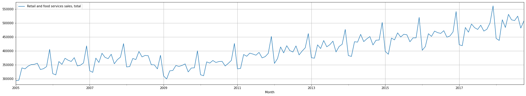

Convert the index back to date again

再次将索引转换回日期

monthly_retail_actuals.index = pd.to_datetime(monthly_retail_actuals.index)

3.5.7.2. Decompose Retail and food services sales, total time series data

3.5.7.2。分解零售和食品服务销售，总时间序列数据

Decomposition is primarily used for time series analysis, and as an analysis tool it can be used to inform forecasting models on your problem. It provides a structured way of thinking about a time series forecasting problem, both generally in terms of modeling complexity and specifically in terms of how-to best capture each of these components in a given model. Multiplicative model was chosen since changes increase or decrease over time whereas Additive model changes over time are consistently made by the same amount.

分解主要用于时间序列分析，并且作为分析工具，可以用于告知问题的预测模型。它提供了一种有关时间序列预测问题的结构化思考方式，通常是从建模复杂性方面，还是从如何最好地捕获给定模型中的每个组件方面。之所以选择乘法模型，是因为随着时间的变化会增加或减少，而随着时间的推移，可加性模型的变化将始终保持相同的数量。

We can see that the trend and seasonality information extracted from the Retail and food services sales, total data does seem consistent with observed data. The residuals seems interesting where variability shows high variability in 2008/2009 (i.e., Great Recession) and in 2012 (Not sure what happened in 2012 — maybe start of booming economy).

我们可以看到，从零售和食品服务销售中提取的趋势和季节性信息的总数据似乎与观察到的数据一致。在2008/2009年(即大萧条)和2012年(不确定2012年发生了什么—可能是经济蓬勃发展)的高变异性中，残差似乎很有趣。

Retail_and_food_services_sales_total_decompose_result = seasonal_decompose(monthly_retail_actuals['Retail and food services sales, total'], model='multiplicative')
Retail_and_food_services_sales_total_decompose_result.plot()
plt.pyplot.show()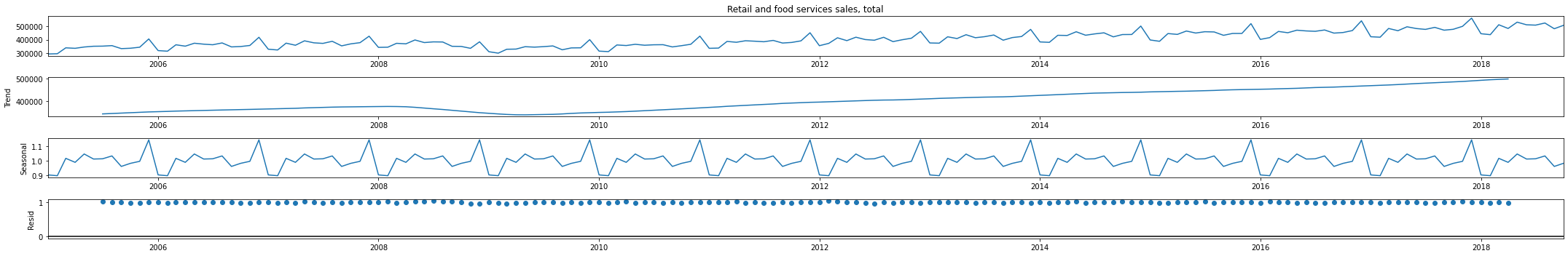

3.5.7.3. Stationary Data Test — Retail and food services sales, total time series data

3.5.7.3。固定数据测试-零售和食品服务销售，总时间序列数据

Check if statistical properties of retail sales series are same. Only then we can forecast that retail sales will be the same in the future as they have been in the past!

检查零售系列的统计属性是否相同。只有这样，我们才能预测未来的零售额将与过去一样！

3.5.7.3.1. ADF Test

3.5.7.3.1。 ADF测试

Augmented Dickey Fuller test (ADF Test) is a common statistical test used to test whether a given Time series is stationary or not

增强Dickey Fuller测试(ADF测试)是一种常用的统计测试，用于测试给定的时间序列是否平稳

adf_test = ADFTest(alpha=0.05)
p_val, should_diff = adf_test.should_diff(monthly_retail_actuals['Retail and food services sales, total']) 

if p_val < 0.05:
    print('Time Series is stationary. p-value is ',  p_val)
else:
    print('Time Series is not stationary. p-value is ',  p_val, '. Differencing is needed: ', should_diff)Time Series is not stationary. p-value is  0.450927778236071 . Differencing is needed:  True

3.5.7.3.2. Estimate number of differences for ARIMA, if time series data is not stationary

3.5.7.3.2。如果时间序列数据不稳定，则估算ARIMA的差异数

from pmdarima.arima.utils import ndiffs

# Estimate the number of differences using an ADF test:
n_adf = ndiffs(monthly_retail_actuals['Retail and food services sales, total'], test='adf') 
print('n_adf:', n_adf)

# Or a KPSS test (auto_arima default):
n_kpss = ndiffs(monthly_retail_actuals['Retail and food services sales, total'], test='kpss') 
print('n_kpss:', n_kpss)

if n_adf == 1 & n_kpss == 1:
    print('Use differencing value of 1 when creating ARIMA model')    
else:
    print('Differencing is not needed when creating ARIMA model')n_adf: 1
n_kpss: 1
Use differencing value of 1 when creating ARIMA model

Based on above. we will be using ‘d’ = 1 when we are creating ARIMA model.

基于以上。创建ARIMA模型时，我们将使用'd'= 1。

3.5.8. Retail sales and food services excl motor vehicle and parts

3.5.8。零售和食品服务，不包括机动车和零件

3.5.8.1. Chart Retail sales and food services excl motor vehicle and parts

3.5.8.1。图表零售和食品服务，不包括机动车和零件

We cannot create a chart using index column so we will be temporarily removing date index before creating line chart with grid. You can create pretty chart with python, but this will do for now.

我们无法使用索引列创建图表，因此在使用网格创建折线图之前，我们将暂时删除日期索引。您可以使用python创建漂亮的图表，但是现在就可以了。

monthly_retail_actuals.reset_index().plot(x='Month', y='Retail sales and food services excl motor vehicle and parts', kind='line', grid=1)
plt.pyplot.show()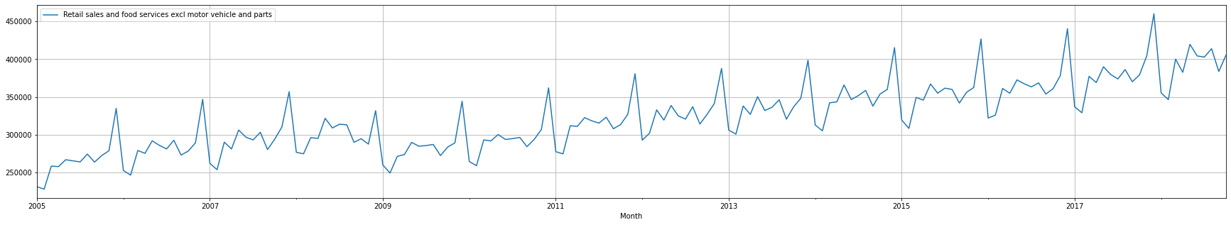

Convert the index to date again.

再次将索引转换为日期。

monthly_retail_actuals.index = pd.to_datetime(monthly_retail_actuals.index)

3.5.8.2. Decompose Retail sales and food services excl motor vehicle and parts time series data

3.5.8.2。分解零售和食品服务(不包括机动车和零件时间序列数据)

Retail_sales_and_food_services_excl_motor_vehicle_and_parts_decompose_result = seasonal_decompose(monthly_retail_actuals['Retail sales and food services excl motor vehicle and parts'], model='multiplicative')
Retail_sales_and_food_services_excl_motor_vehicle_and_parts_decompose_result.plot()
plt.pyplot.show()

3.5.8.3. Stationary Data Test — Retail and food services sales, total time series data

3.5.8.3。固定数据测试-零售和食品服务销售，总时间序列数据

3.5.8.3.1. ADF Test

3.5.8.3.1。 ADF测试

Augmented Dickey Fuller test (ADF Test) is a common statistical test used to test whether a given Time series is stationary or not

增强Dickey Fuller测试(ADF测试)是一种常用的统计测试，用于测试给定的时间序列是否平稳

adf_test = ADFTest(alpha=0.05)
p_val, should_diff = adf_test.should_diff(monthly_retail_actuals['Retail sales and food services excl motor vehicle and parts']) 

if p_val < 0.05:
    print('Time Series is stationary. p-value is ',  p_val)
else:
    print('Time Series is not stationary. p-value is ',  p_val, '. Differencing is needed: ', should_diff)Time Series is stationary. p-value is  0.04572401345436711

3.5.8.3.2. Estimate number of differences for ARIMA, if time series data is not stationary

3.5.8.3.2。如果时间序列数据不稳定，则估算ARIMA的差异数

from pmdarima.arima.utils import ndiffs

# Estimate the number of differences using an ADF test:
n_adf = ndiffs(monthly_retail_actuals['Retail sales and food services excl motor vehicle and parts'], test='adf') 
print('n_adf:', n_adf)

# Or a KPSS test (auto_arima default):
n_kpss = ndiffs(monthly_retail_actuals['Retail sales and food services excl motor vehicle and parts'], test='kpss') 
print('n_kpss:',n_kpss)

if n_adf == 1 & n_kpss == 1:
    print('Use differencing value of 1 when creating ARIMA model')    
else:
    print('Differencing is not needed when creating ARIMA model')n_adf: 0
n_kpss: 1
Differencing is not needed when creating ARIMA model

3.5.9. Retail sales and food services excl gasoline stations

3.5.9。零售和食品服务，不包括加油站

3.5.9.1. Chart Retail sales and food services excl gasoline stations

3.5.9.1。零售和食品服务图表，不包括加油站

We cannot create a chart using index column so we will be temporarily removing date index before creating line chart with grid. You can create pretty chart with python, but this will do for now.

我们无法使用索引列创建图表，因此在使用网格创建折线图之前，我们将暂时删除日期索引。您可以使用python创建漂亮的图表，但是现在就可以了。

monthly_retail_actuals.reset_index().plot(x='Month', y='Retail sales and food services excl gasoline stations', kind='line', grid=1)
plt.pyplot.show()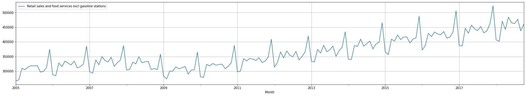

Convert the index to date again.

再次将索引转换为日期。

monthly_retail_actuals.index = pd.to_datetime(monthly_retail_actuals.index)

3.5.9.2. Decompose Retail sales and food services excl gasoline stations time series data

3.5.9.2。分解零售和食品服务(不包括加油站)时间序列数据

Retail_sales_and_food_services_excl_gasoline_stations_decompose_result = seasonal_decompose(monthly_retail_actuals['Retail sales and food services excl gasoline stations'], model='multiplicative')
Retail_sales_and_food_services_excl_gasoline_stations_decompose_result.plot()
plt.pyplot.show()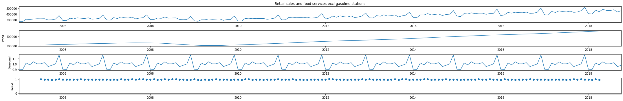

3.5.9.3. Stationary Data Test — Retail and food services sales, total time series data

3.5.9.3。固定数据测试-零售和食品服务销售，总时间序列数据

3.5.9.3.1. ADF Test

3.5.9.3.1。 ADF测试

Augmented Dickey Fuller test (ADF Test) is a common statistical test used to test whether a given Time series is stationary or not

增强Dickey Fuller测试(ADF测试)是一种常用的统计测试，用于测试给定的时间序列是否平稳

adf_test = ADFTest(alpha=0.05)
p_val, should_diff = adf_test.should_diff(monthly_retail_actuals['Retail sales and food services excl gasoline stations']) 

if p_val < 0.05:
    print('Time Series is stationary. p-value is ',  p_val)
else:
    print('Time Series is not stationary. p-value is ',  p_val, '. Differencing is needed: ', should_diff)Time Series is not stationary. p-value is  0.6406252363274619 . Differencing is needed:  True

3.5.9.3.2. Estimate number of differences for ARIMA, if time series data is not stationary

3.5.9.3.2。如果时间序列数据不稳定，则估算ARIMA的差异数

from pmdarima.arima.utils import ndiffs

# Estimate the number of differences using an ADF test:
n_adf = ndiffs(monthly_retail_actuals['Retail sales and food services excl gasoline stations'], test='adf') 
print('n_adf:', n_adf)

# Or a KPSS test (auto_arima default):
n_kpss = ndiffs(monthly_retail_actuals['Retail sales and food services excl gasoline stations'], test='kpss') 
print('n_kpss:',n_kpss)

if n_adf == 1 & n_kpss == 1:
    print('Use differencing value of 1 when creating ARIMA model')    
else:
    print('Differencing is not needed when creating ARIMA model')n_adf: 1
n_kpss: 1
Use differencing value of 1 when creating ARIMA model

3.5.10. Retail sales and food services excl motor vehicle and parts and gasoline stations

3.5.10。零售和食品服务，不包括机动车，零件和加油站

3.5.10.1. Chart Retail sales and food services excl motor vehicle and parts and gasoline stations

3.5.10.1。图表零售和食品服务，不包括汽车，零件和加油站

We cannot create a chart using index column so we will be temporarily removing date index before creating line chart with grid. You can create really pretty chart with python, but this will do for now.

我们无法使用索引列创建图表，因此在使用网格创建折线图之前，我们将暂时删除日期索引。您可以使用python创建非常漂亮的图表，但是现在就可以了。

monthly_retail_actuals.reset_index().plot(x='Month', y='Retail sales and food services excl motor vehicle and parts and gasoline stations', kind='line', grid=1)
plt.pyplot.show()

Convert the index to date again

再次将索引转换为日期

monthly_retail_actuals.index = pd.to_datetime(monthly_retail_actuals.index)

3.5.10.2. Decompose Retail sales and food services excl motor vehicle and parts and gasoline stations time series data

3.5.10.2。分解零售和食品服务(不包括汽车，零件和加油站)的时间序列数据

Retail_sales_and_food_services_excl_motor_vehicle_and_parts_and_gasoline_stations_decompose_result = seasonal_decompose(monthly_retail_actuals['Retail sales and food services excl motor vehicle and parts and gasoline stations'], model='multiplicative')
Retail_sales_and_food_services_excl_motor_vehicle_and_parts_and_gasoline_stations_decompose_result.plot()
plt.pyplot.show()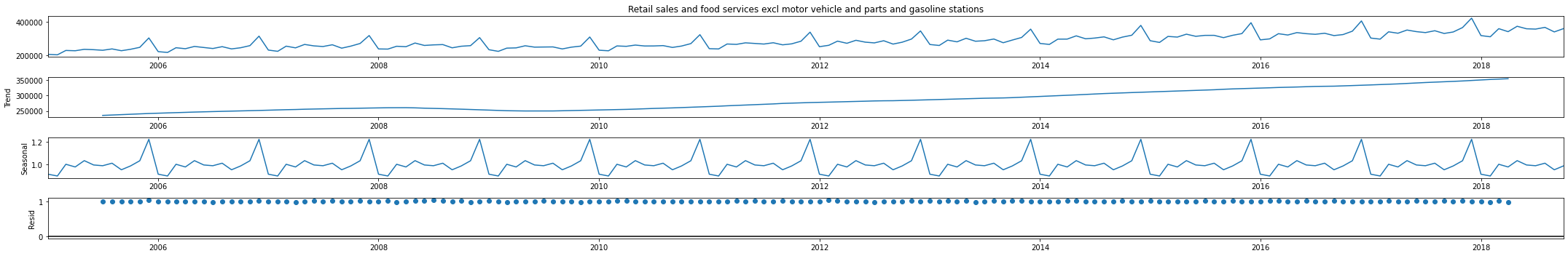

3.5.10.3. Stationary Data Test — Retail and food services sales, total time series data

3.5.10.3。固定数据测试-零售和食品服务销售，总时间序列数据

Check if statistical properties of retail sales series are same. Only then we can forecast that retail sales will be the same in the future as they have been in the past!

检查零售系列的统计属性是否相同。只有这样，我们才能预测未来的零售额将与过去一样！

3.5.10.3.1. ADF Test

3.5.10.3.1。 ADF测试

Augmented Dickey Fuller test (ADF Test) is a common statistical test used to test whether a given Time series is stationary or not

增强Dickey Fuller测试(ADF测试)是一种常用的统计测试，用于测试给定的时间序列是否平稳

adf_test = ADFTest(alpha=0.05)
p_val, should_diff = adf_test.should_diff(monthly_retail_actuals['Retail sales and food services excl motor vehicle and parts and gasoline stations']) 

if p_val < 0.05:
    print('Time Series is stationary. p-value is ',  p_val)
else:
    print('Time Series is not stationary. p-value is ',  p_val, '. Differencing is needed: ', should_diff)Time Series is not stationary. p-value is  0.08047159609506416 . Differencing is needed:  True

3.5.10.3.2. Estimate number of differences for ARIMA, if time series data is not stationary

3.5.10.3.2。如果时间序列数据不稳定，则估算ARIMA的差异数

from pmdarima.arima.utils import ndiffs

# Estimate the number of differences using an ADF test:
n_adf = ndiffs(monthly_retail_actuals['Retail sales and food services excl motor vehicle and parts and gasoline stations'], test='adf') 
print('n_adf:', n_adf)

# Or a KPSS test (auto_arima default):
n_kpss = ndiffs(monthly_retail_actuals['Retail sales and food services excl motor vehicle and parts and gasoline stations'], test='kpss') 
print('n_kpss:',n_kpss)

if n_adf == 1 & n_kpss == 1:
    print('Use differencing value of 1 when creating ARIMA model')    
else:
    print('Differencing is not needed when creating ARIMA model')n_adf: 1
n_kpss: 1
Use differcening value of 1 when creating ARIMA model

3.5.11. Retail sales, total

3.5.11。零售总额

3.5.11.1. Chart Retail sales, total

3.5.11.1。图表零售总额

monthly_retail_actuals.reset_index().plot(x='Month', y='Retail sales, total', kind='line', grid=1)
plt.pyplot.show()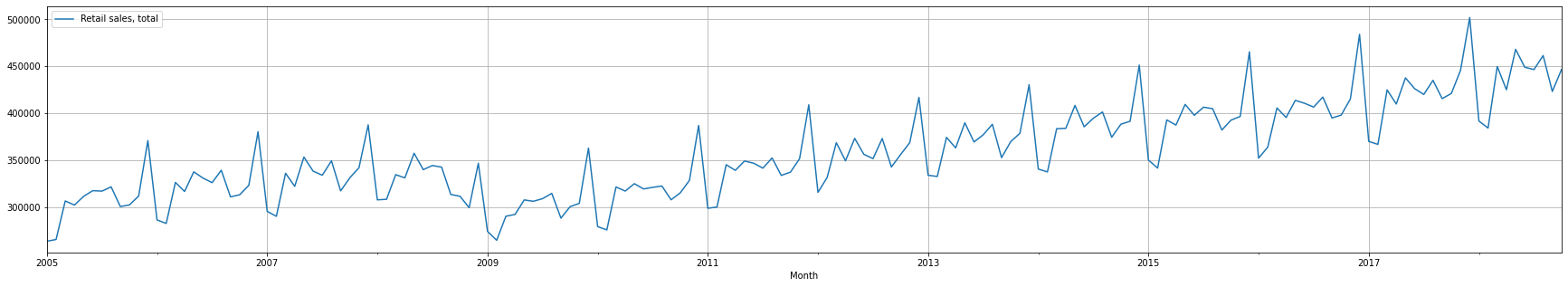

Convert the index to date again

再次将索引转换为日期

monthly_retail_actuals.index = pd.to_datetime(monthly_retail_actuals.index)

3.5.11.2. Decompose Retail sales, total time series data

3.5.11.2。分解零售，总时间序列数据

Retail_sales_total_decompose_result = seasonal_decompose(monthly_retail_actuals['Retail sales, total'], model='multiplicative')
Retail_sales_total_decompose_result.plot()
plt.pyplot.show()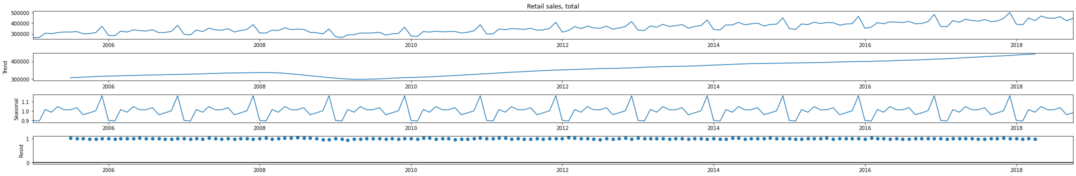

3.5.11.3. Stationary Data Test — Retail and food services sales, total time series data

3.5.11.3。固定数据测试-零售和食品服务销售，总时间序列数据

Check if statistical properties of retail sales series are same. Only then we can forecast that retail sales will be the same in the future as they have been in the past!

检查零售系列的统计属性是否相同。只有这样，我们才能预测未来的零售额将与过去一样！

3.5.11.3.1. ADF Test

3.5.11.3.1。 ADF测试

Augmented Dickey Fuller test (ADF Test) is a common statistical test used to test whether a given Time series is stationary or not

增强Dickey Fuller测试(ADF测试)是一种常用的统计测试，用于测试给定的时间序列是否平稳

adf_test = ADFTest(alpha=0.05)
p_val, should_diff = adf_test.should_diff(monthly_retail_actuals['Retail sales, total']) 

if p_val < 0.05:
    print('Time Series is stationary. p-value is ',  p_val)
else:
    print('Time Series is not stationary. p-value is ',  p_val, '. Differencing is needed: ', should_diff)Time Series is not stationary. p-value is  0.43936588714000624 . Differencing is needed:  True

3.5.11.3.2. Estimate number of differences for ARIMA, if time series data is not stationary

3.5.11.3.2。如果时间序列数据不稳定，则估算ARIMA的差异数

from pmdarima.arima.utils import ndiffs

# Estimate the number of differences using an ADF test:
n_adf = ndiffs(monthly_retail_actuals['Retail sales, total'], test='adf') 
print('n_adf:', n_adf)

# Or a KPSS test (auto_arima default):
n_kpss = ndiffs(monthly_retail_actuals['Retail sales, total'], test='kpss') 
print('n_kpss:',n_kpss)

if n_adf == 1 & n_kpss == 1:
    print('Use differencing value of 1 when creating ARIMA model')    
else:
    print('Differencing is not needed when creating ARIMA model')n_adf: 1
n_kpss: 1
Use differencing value of 1 when creating ARIMA model

3.5.12. Retail sales, total (excl. motor vehicle and parts dealers)

3.5.12。零售总额(不包括汽车和零件经销商)

3.5.12.1. Chart Retail sales, total (excl. motor vehicle and parts dealers)

3.5.12.1。图表零售总额(不包括汽车和零件经销商)

We cannot create a chart using index column so we will be temporarily removing date index before creating line chart with grid. You can create pretty chart with python, but this will do for now.

我们无法使用索引列创建图表，因此在使用网格创建折线图之前，我们将暂时删除日期索引。您可以使用python创建漂亮的图表，但是现在就可以了。

monthly_retail_actuals.reset_index().plot(x='Month', y='Retail sales, total (excl. motor vehicle and parts dealers)', kind='line', grid=1)
plt.pyplot.show()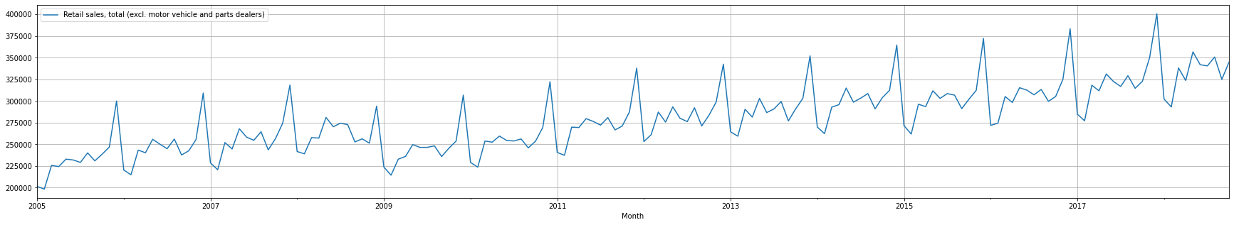

Convert the index to date again.

再次将索引转换为日期。

monthly_retail_actuals.index = pd.to_datetime(monthly_retail_actuals.index)

3.5.12.2. Decompose Retail sales, total (excl. motor vehicle and parts dealers) time series data

3.5.12.2。分解零售，总时间(不包括汽车和零件经销商)的时间序列数据

Retail_sales_total_excl_motor_vehicle_and_parts_dealers_decompose_result = seasonal_decompose(monthly_retail_actuals['Retail sales, total (excl. motor vehicle and parts dealers)'], model='multiplicative')
Retail_sales_total_excl_motor_vehicle_and_parts_dealers_decompose_result.plot()
plt.pyplot.show()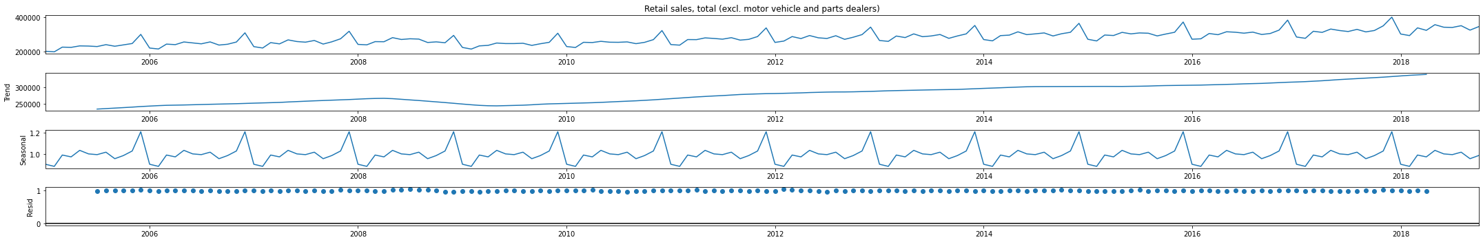

3.5.12.3. Stationary Data Test — Retail and food services sales, total time series data

3.5.12.3。固定数据测试-零售和食品服务销售，总时间序列数据

Check if statistical properties of retail sales series are same. Only then we can forecast that retail sales will be the same in the future as they have been in the past!

检查零售系列的统计属性是否相同。只有这样，我们才能预测未来的零售额将与过去一样！

3.5.12.3.1. ADF Test

3.5.12.3.1。 ADF测试

Augmented Dickey Fuller test (ADF Test) is a common statistical test used to test whether a given Time series is stationary or not

增强Dickey Fuller测试(ADF测试)是一种常用的统计测试，用于测试给定的时间序列是否平稳

adf_test = ADFTest(alpha=0.05)
p_val, should_diff = adf_test.should_diff(monthly_retail_actuals['Retail sales, total (excl. motor vehicle and parts dealers)']) 

if p_val < 0.05:
    print('Time Series is stationary. p-value is ',  p_val)
else:
    print('Time Series is not stationary. p-value is ',  p_val, '. Differencing is needed: ', should_diff)Time Series is stationary. p-value is  0.015901175253013197

3.5.12.3.2. Estimate number of differences for ARIMA, if time series data is not stationary

3.5.12.3.2。如果时间序列数据不稳定，则估算ARIMA的差异数

from pmdarima.arima.utils import ndiffs

# Estimate the number of differences using an ADF test:
n_adf = ndiffs(monthly_retail_actuals['Retail sales, total (excl. motor vehicle and parts dealers)'], test='adf') 
print('n_adf:', n_adf)

# Or a KPSS test (auto_arima default):
n_kpss = ndiffs(monthly_retail_actuals['Retail sales, total (excl. motor vehicle and parts dealers)'], test='kpss') 
print('n_kpss:',n_kpss)

if n_adf == 1 & n_kpss == 1:
    print('Use differencing value of 1 when creating ARIMA model')    
else:
    print('Differencing is not needed when creating ARIMA model')n_adf: 0
n_kpss: 1
Differencing is not needed when creating ARIMA model

3.6。准备数据 (3.6. Prep Data)

We will need to prep data to ensure we only use clean data to create our forecast. Some of the basic data prep tasks are:

我们将需要准备数据以确保仅使用干净数据来创建预测。一些基本的数据准备任务是：

Remove data outliers. Let say for one month, your sales doubled or tripled due to once in lifetime promotion. This is nice data point to consider, but it will skew our forecast without providing any value. We will need to cap and floor our data to ensure outliers are removed.
删除数据异常值。假设一个月内，由于终身促销一次，您的销售额翻了一番或三倍。这是可以考虑的很好的数据点，但是它会扭曲我们的预测而没有提供任何价值。我们将需要对数据进行上限和下限以确保消除异常值。
Impute missing data. Sometimes, some of the data are just missing for whatever the reason. If the percentage of missing value is low, then you can impute that missing data.
估算缺少的数据。有时，无论出于何种原因，一些数据都会丢失。如果缺失值的百分比较低，则可以估算该缺失数据。

Monthly Trade Report does not seem to have any outliers nor missing data, so this step is not need.

每月贸易报告似乎没有异常值或数据缺失，因此不需要此步骤。

3.7。开发和验证预测模型 (3.7. Develop and Validate Forecast Model)

To create a forecast model, we shall use ARIMA algorithm to analyzes the data, looking for specific types of patterns or trends. The ARIMA algorithm then uses the results of this analysis over many iterations to find the optimal (hyper) parameters for creating the forecast model. These parameters are then applied across the entire data set to develop a forecast model.

要创建预测模型，我们将使用ARIMA算法分析数据，寻找特定类型的模式或趋势。然后，ARIMA算法在多次迭代中使用此分析的结果，以找到用于创建预测模型的最佳(超级)参数。然后，将这些参数应用于整个数据集以建立预测模型。

3.7.1. Retail and food services sales, total

3.7.1。零售和食品服务销售额，总计

3.7.1.1. Filter Monthly Retail Data to just Retail and food services sales, total data

3.7.1.1。将每月零售数据过滤为仅零售和食品服务销售，总数据

Retail_and_food_services_sales_total_data = monthly_retail_actuals.filter(items=['Retail and food services sales, total'])print('All: ', Retail_and_food_services_sales_total_data.shape)All:  (166, 1)

3.7.1.2. Split the data into Train and Test data

3.7.1.2。将数据分为训练和测试数据

We will be diving data into two sets of data:

我们将把数据分为两组数据：

Train Data
火车数据
Test Data
测试数据

Usually we use 70 Train/30 Test (70/30) split, 80 Train/20 Test (80/20) split, 90 Train/10 Test (90/10) split or even 95 Train/5 Test (95/5) where train data is used to create a forecast and test data is used to validate the forecast. For simplification purposes, we shall split the data as follows:

通常我们使用70 Train / 30 Test(70/30)split，80 Train / 20 Test(80/20)split，90 Train / 10 Test(90/10)split甚至是95 Train / 5 Test(95/5)火车数据用于创建预测，测试数据用于验证预测。为了简化起见，我们将数据拆分如下：

Train Data: January 2005 thru December 2016
火车数据：2005年1月至2016年12月
Test Data: January 2017 thru October 2018
测试数据：2017年1月至2018年10月

Retail_and_food_services_sales_total_train = Retail_and_food_services_sales_total_data.loc['2005-01-01':'2016-12-01']
Retail_and_food_services_sales_total_test = Retail_and_food_services_sales_total_data.loc['2017-01-01':]

3.7.1.3. Validate data split was done correctly

3.7.1.3。验证数据分割是否正确完成

print( 'Train: ', Retail_and_food_services_sales_total_train.shape)
print( 'Test: ', Retail_and_food_services_sales_total_test.shape)Train:  (144, 1)
Test:  (22, 1)

3.7.1.4. Train Forecast Model for Retail and food services sales, total using ARIMA (Autoregressive Integrated Moving Average) Model to find optimal Hyper-Parameters

3.7.1.4。训练零售和食品服务销售的预测模型，使用ARIMA(自回归综合移动平均线)模型进行总预测以找到最佳的超参数

ARIMA Model is bit difficult to explain, but it is best way to create a forecast of times series data. If you want to know more, here goes:

ARIMA模型有点难以解释，但它是创建时间序列数据预测的最佳方法。如果您想了解更多，这里有：

AR: Autoregression. A model that uses the dependent relationship between an observation and some number of lagged observations.
AR：自回归。一种模型，它使用观察值和一些滞后观察值之间的依赖关系。
I: Integrated. The use of differencing of raw observations (e.g. subtracting an observation from an observation at the previous time step) in order to make the time series stationary.
一：集成。为了使时间序列固定，使用原始观测值的差异(例如，从上一个时间步长的观测值中减去观测值)。
MA: Moving Average. A model that uses the dependency between an observation and a residual error from a moving average model applied to lagged observations.
MA：移动平均线。一种模型，该模型使用观察值与应用于滞后观察值的移动平均模型的残差之间的依赖关系。

Since we are too lazy (well, I am) to understand inner workings of fine tuning ARIMA model to find the best fit for our needs, we will be using something called Auto(mated) ARIMA or auto_arima as shown below. Just pass the train data and let it find the best fit for our needs.

由于我们太懒惰(好吧，我)无法理解ARIMA模型微调的内部工作原理，无法找到最适合我们需求的模型，因此我们将使用一种称为Auto(mated)ARIMA或auto_arima的方法，如下所示。只需传递火车数据，并使其最适合我们的需求即可。

3.7.1.4.1. Find the best fit using brute force search using train data

3.7.1.4.1。通过使用火车数据的蛮力搜索找到最合适的

Please note the parameters used:

请注意使用的参数：

m=12 (Denote that retail sales data is monthly)
m = 12(表示每月零售数据)
seasonal=True (Denotes that retail sales data has seasonality)
Seasons = True(表示零售数据具有季节性)
d=1 (Denotes that retail sales data is not stationary and differencing of 1 is required as noted on section 3.5.7.3)
d = 1(表示零售数据不稳定，如3.5.7.3节所述，要求相差1)。
stepwise=False (Denotes brute force search since dateset is small, not intelligent search)
stepwise = False(由于日期集很小，因此不是智能搜索，表示蛮力搜索)

Retail_and_food_services_sales_total_fit = pm.auto_arima(Retail_and_food_services_sales_total_train, 
                           m=12,
                           seasonal=True,
                           d=1,
                           trace=True,
                           error_action='ignore',  
                           suppress_warnings=True, 
                           stepwise=False)ARIMA(0,1,0)(0,1,0)[12]             : AIC=2759.906, Time=0.05 sec
 ARIMA(0,1,0)(0,1,1)[12]             : AIC=2763.700, Time=0.31 sec
 ARIMA(0,1,0)(0,1,2)[12]             : AIC=2761.164, Time=0.75 sec
 ARIMA(0,1,0)(1,1,0)[12]             : AIC=2761.588, Time=0.15 sec
 ARIMA(0,1,0)(1,1,1)[12]             : AIC=2766.404, Time=0.46 sec
 ARIMA(0,1,0)(1,1,2)[12]             : AIC=2760.336, Time=1.19 sec
 ARIMA(0,1,0)(2,1,0)[12]             : AIC=2761.317, Time=0.56 sec
 ARIMA(0,1,0)(2,1,1)[12]             : AIC=2766.507, Time=1.58 sec
 ARIMA(0,1,0)(2,1,2)[12]             : AIC=2758.753, Time=3.74 sec
 ARIMA(0,1,1)(0,1,0)[12]             : AIC=2762.290, Time=0.08 sec
 ARIMA(0,1,1)(0,1,1)[12]             : AIC=2764.271, Time=0.44 sec
 ARIMA(0,1,1)(0,1,2)[12]             : AIC=2763.623, Time=1.04 sec
 ARIMA(0,1,1)(1,1,0)[12]             : AIC=2764.273, Time=0.27 sec
 ARIMA(0,1,1)(1,1,1)[12]             : AIC=2764.205, Time=0.86 sec
 ARIMA(0,1,1)(1,1,2)[12]             : AIC=2762.501, Time=1.98 sec
 ARIMA(0,1,1)(2,1,0)[12]             : AIC=2763.804, Time=0.85 sec
 ARIMA(0,1,1)(2,1,1)[12]             : AIC=2762.004, Time=1.81 sec
 ARIMA(0,1,1)(2,1,2)[12]             : AIC=2760.362, Time=5.84 sec
 ARIMA(0,1,2)(0,1,0)[12]             : AIC=2763.647, Time=0.24 sec
 ARIMA(0,1,2)(0,1,1)[12]             : AIC=2765.645, Time=0.51 sec
 ARIMA(0,1,2)(0,1,2)[12]             : AIC=2764.985, Time=1.34 sec
 ARIMA(0,1,2)(1,1,0)[12]             : AIC=2765.645, Time=0.32 sec
 ARIMA(0,1,2)(1,1,1)[12]             : AIC=2765.314, Time=1.05 sec
 ARIMA(0,1,2)(1,1,2)[12]             : AIC=2763.855, Time=2.00 sec
 ARIMA(0,1,2)(2,1,0)[12]             : AIC=2765.207, Time=0.97 sec
 ARIMA(0,1,2)(2,1,1)[12]             : AIC=2763.391, Time=2.19 sec
 ARIMA(0,1,3)(0,1,0)[12]             : AIC=2762.732, Time=0.36 sec
 ARIMA(0,1,3)(0,1,1)[12]             : AIC=2764.731, Time=0.64 sec
 ARIMA(0,1,3)(0,1,2)[12]             : AIC=2764.387, Time=1.51 sec
 ARIMA(0,1,3)(1,1,0)[12]             : AIC=2764.731, Time=0.42 sec
 ARIMA(0,1,3)(1,1,1)[12]             : AIC=2764.470, Time=1.42 sec
 ARIMA(0,1,3)(2,1,0)[12]             : AIC=2764.599, Time=1.21 sec
 ARIMA(0,1,4)(0,1,0)[12]             : AIC=2761.432, Time=0.20 sec
 ARIMA(0,1,4)(0,1,1)[12]             : AIC=2763.425, Time=0.83 sec
 ARIMA(0,1,4)(1,1,0)[12]             : AIC=2763.425, Time=0.48 sec
 ARIMA(0,1,5)(0,1,0)[12]             : AIC=2761.100, Time=0.30 sec
 ARIMA(1,1,0)(0,1,0)[12]             : AIC=2762.752, Time=0.07 sec
 ARIMA(1,1,0)(0,1,1)[12]             : AIC=2764.733, Time=1.36 sec
 ARIMA(1,1,0)(0,1,2)[12]             : AIC=2764.018, Time=0.97 sec
 ARIMA(1,1,0)(1,1,0)[12]             : AIC=2764.734, Time=0.29 sec
 ARIMA(1,1,0)(1,1,1)[12]             : AIC=2764.618, Time=0.72 sec
 ARIMA(1,1,0)(1,1,2)[12]             : AIC=2762.817, Time=1.82 sec
 ARIMA(1,1,0)(2,1,0)[12]             : AIC=2764.203, Time=1.21 sec
 ARIMA(1,1,0)(2,1,1)[12]             : AIC=2762.306, Time=1.80 sec
 ARIMA(1,1,0)(2,1,2)[12]             : AIC=2760.560, Time=4.89 sec
 ARIMA(1,1,1)(0,1,0)[12]             : AIC=2764.512, Time=0.39 sec
 ARIMA(1,1,1)(0,1,1)[12]             : AIC=2766.497, Time=1.30 sec
 ARIMA(1,1,1)(0,1,2)[12]             : AIC=2765.789, Time=3.70 sec
 ARIMA(1,1,1)(1,1,0)[12]             : AIC=2766.498, Time=0.76 sec
 ARIMA(1,1,1)(1,1,1)[12]             : AIC=2766.335, Time=1.54 sec
 ARIMA(1,1,1)(1,1,2)[12]             : AIC=2764.604, Time=3.85 sec
 ARIMA(1,1,1)(2,1,0)[12]             : AIC=2765.983, Time=3.22 sec
 ARIMA(1,1,1)(2,1,1)[12]             : AIC=2764.104, Time=4.55 sec
 ARIMA(1,1,2)(0,1,0)[12]             : AIC=2762.359, Time=0.48 sec
 ARIMA(1,1,2)(0,1,1)[12]             : AIC=2764.357, Time=1.12 sec
 ARIMA(1,1,2)(0,1,2)[12]             : AIC=2763.772, Time=3.64 sec
 ARIMA(1,1,2)(1,1,0)[12]             : AIC=2764.357, Time=1.54 sec
 ARIMA(1,1,2)(1,1,1)[12]             : AIC=2763.862, Time=2.36 sec
 ARIMA(1,1,2)(2,1,0)[12]             : AIC=2764.015, Time=3.54 sec
 ARIMA(1,1,3)(0,1,0)[12]             : AIC=2762.752, Time=0.55 sec
 ARIMA(1,1,3)(0,1,1)[12]             : AIC=2764.749, Time=2.10 sec
 ARIMA(1,1,3)(1,1,0)[12]             : AIC=2764.750, Time=1.45 sec
 ARIMA(1,1,4)(0,1,0)[12]             : AIC=2762.944, Time=0.81 sec
 ARIMA(2,1,0)(0,1,0)[12]             : AIC=2764.830, Time=0.16 sec
 ARIMA(2,1,0)(0,1,1)[12]             : AIC=2766.827, Time=0.43 sec
 ARIMA(2,1,0)(0,1,2)[12]             : AIC=2765.992, Time=1.16 sec
 ARIMA(2,1,0)(1,1,0)[12]             : AIC=2766.827, Time=0.79 sec
 ARIMA(2,1,0)(1,1,1)[12]             : AIC=2766.346, Time=1.18 sec
 ARIMA(2,1,0)(1,1,2)[12]             : AIC=2764.658, Time=2.23 sec
 ARIMA(2,1,0)(2,1,0)[12]             : AIC=2766.229, Time=1.12 sec
 ARIMA(2,1,0)(2,1,1)[12]             : AIC=2764.162, Time=2.91 sec
 ARIMA(2,1,1)(0,1,0)[12]             : AIC=2765.373, Time=0.38 sec
 ARIMA(2,1,1)(0,1,1)[12]             : AIC=2767.367, Time=1.75 sec
 ARIMA(2,1,1)(0,1,2)[12]             : AIC=2766.411, Time=3.37 sec
 ARIMA(2,1,1)(1,1,0)[12]             : AIC=2767.367, Time=2.00 sec
 ARIMA(2,1,1)(1,1,1)[12]             : AIC=2766.449, Time=2.59 sec
 ARIMA(2,1,1)(2,1,0)[12]             : AIC=2766.701, Time=4.82 sec
 ARIMA(2,1,2)(0,1,0)[12]             : AIC=2713.459, Time=1.06 sec
 ARIMA(2,1,2)(0,1,1)[12]             : AIC=2715.773, Time=3.49 sec
 ARIMA(2,1,2)(1,1,0)[12]             : AIC=2715.772, Time=3.75 sec
 ARIMA(2,1,3)(0,1,0)[12]             : AIC=2715.442, Time=1.00 sec
 ARIMA(3,1,0)(0,1,0)[12]             : AIC=2766.043, Time=0.15 sec
 ARIMA(3,1,0)(0,1,1)[12]             : AIC=2768.043, Time=0.48 sec
 ARIMA(3,1,0)(0,1,2)[12]             : AIC=2767.327, Time=1.34 sec
 ARIMA(3,1,0)(1,1,0)[12]             : AIC=2768.043, Time=0.55 sec
 ARIMA(3,1,0)(1,1,1)[12]             : AIC=2767.463, Time=1.25 sec
 ARIMA(3,1,0)(2,1,0)[12]             : AIC=2767.567, Time=1.40 sec
 ARIMA(3,1,1)(0,1,0)[12]             : AIC=2764.669, Time=0.64 sec
 ARIMA(3,1,1)(0,1,1)[12]             : AIC=2766.662, Time=2.34 sec
 ARIMA(3,1,1)(1,1,0)[12]             : AIC=2766.663, Time=1.29 sec
 ARIMA(3,1,2)(0,1,0)[12]             : AIC=2714.518, Time=1.23 sec
 ARIMA(4,1,0)(0,1,0)[12]             : AIC=2763.900, Time=0.24 sec
 ARIMA(4,1,0)(0,1,1)[12]             : AIC=2765.883, Time=0.69 sec
 ARIMA(4,1,0)(1,1,0)[12]             : AIC=2765.884, Time=1.13 sec
 ARIMA(4,1,1)(0,1,0)[12]             : AIC=2764.851, Time=0.53 sec
 ARIMA(5,1,0)(0,1,0)[12]             : AIC=2762.896, Time=0.33 sec
Total fit time: 135.895 seconds

3.7.1.4.2. View the summary of selected optimal hyper-parameters

3.7.1.4.2。查看所选最佳超参数的摘要

Retail_and_food_services_sales_total_fit.summary()

SARIMAX Results Dep. Variable: y No. Observations: 144 Model: SARIMAX(2, 1, 2)x(0, 1, [], 12) Log Likelihood -1351.730 Date: Sat, 15 Aug 2020 AIC 2713.459 Time: 15:08:17 BIC 2727.835 Sample: 0 HQIC 2719.301–144 Covariance Type: opg coef std err z P>|z| [0.025 0.975] ar.L1 -1.1695 0.009 -125.006 0.000 -1.188 -1.151 ar.L2 -0.9926 0.010 -102.907 0.000 -1.011 -0.974 ma.L1 1.1568 0.036 31.737 0.000 1.085 1.228 ma.L2 0.9960 0.065 15.235 0.000 0.868 1.124 sigma2 6.443e+07 2.38e-10 2.7e+17 0.000 6.44e+07 6.44e+07 Ljung-Box (Q): 48.88 Jarque-Bera (JB): 2.84 Prob(Q): 0.16 Prob(JB): 0.24 Heteroskedasticity (H): 0.78 Skew: -0.18 Prob(H) (two-sided): 0.42 Kurtosis: 3.62 Warnings:[1] Covariance matrix calculated using the outer product of gradients (complex-step).[2] Covariance matrix is singular or near-singular, with condition number 2.23e+33. Standard errors may be unstable.

SARIMAX结果部变量：y号。观测值：144模型：SARIMAX(2，1，2)x(0，1，[]，12)对数似然-1351.730日期：2020年8月15日，星期六AIC 2713.459时间：15:08:17 BIC 2727.835样本：0 HQIC 2719.301–144协方差类型：opg coef std err z P> | z | [0.025 0.975] ar.L1 -1.1695 0.009 -125.006 0.000 -1.188 -1.151 ar.L2 -0.9926 0.010 -102.907 0.000 -1.011 -0.974 ma.L1 1.1568 0.036 31.737 0.000 1.085 1.228 ma.L2 0.9960 0.065 15.235 0.000 0.868 1.124 sigma2 6.443 e + 07 2.38e-10 2.7e + 17 0.000 6.44e + 07 6.44e + 07 Ljung-Box(Q)：48.88 Jarque-Bera(JB)：2.84 Prob(Q)：0.16 Prob(JB)：0.24异方差( H)：0.78倾斜度：-0.18 Prob(H)(两侧)：0.42峰度：3.62警告：[1]使用梯度的外部乘积(复杂步骤)计算的协方差矩阵。[2] 协方差矩阵是奇异的或近似奇异的，条件编号为2.23e + 33。标准错误可能不稳定。

3.7.1.5. Fit Forecast Model

3.7.1.5。拟合预测模型

Now, you have optimal parameters using either stepwise or random. Next step is to call ARIMA function and pass those parameters.

现在，您可以使用逐步或随机的最佳参数。下一步是调用ARIMA函数并传递这些参数。

Retail_and_food_services_sales_total_fit.fit(Retail_and_food_services_sales_total_train)ARIMA(maxiter=50, method='lbfgs', order=(2, 1, 2), out_of_sample_size=0,
      scoring='mse', scoring_args={}, seasonal_order=(0, 1, 0, 12),
      start_params=None, suppress_warnings=True, trend=None,
      with_intercept=False)

3.7.1.6. Predict Forecast

3.7.1.6。预测预报

Using your trained model, predict forecast for next 22 months, starting January 2017.

使用训练有素的模型，预测从2017年1月开始的未来22个月的预测。

Retail_and_food_services_sales_total_forecast = Retail_and_food_services_sales_total_fit.predict(n_periods=22)Retail_and_food_services_sales_total_forecastarray([422261.2511875 , 440888.14330158, 481773.90801362, 472892.78575083,
       496217.76225349, 484826.66043455, 484703.78630138, 497242.44591658,
       468110.4943768 , 476557.81401408, 492189.72208598, 559869.68293006,
       446150.39262897, 464027.68573856, 500716.49972167, 497487.54452719,
       518368.43403657, 504225.30016304, 509746.76022861, 518416.2849135 ,
       488206.59860748, 501754.72992269])

3.7.1.7. Validate Forecast

3.7.1.7。验证预测

3.7.1.7.1. Compare historical/actual sales data with forecast

3.7.1.7.1。比较历史/实际销售数据与预测

Retail_and_food_services_sales_total_validate = pd.DataFrame(Retail_and_food_services_sales_total_forecast, index = Retail_and_food_services_sales_total_test.index, columns=['Prediction'])
Retail_and_food_services_sales_total_validate = pd.concat([Retail_and_food_services_sales_total_test, Retail_and_food_services_sales_total_validate], axis=1)
Retail_and_food_services_sales_total_validate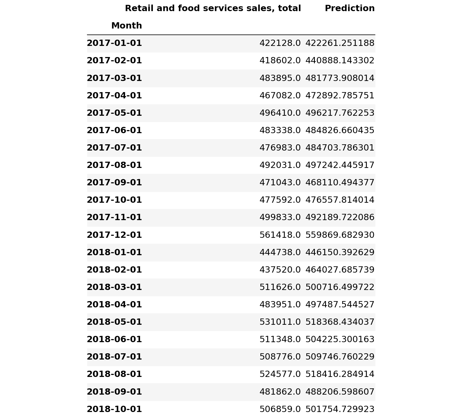

3.7.1.7.2. Plot the differences between historical/actual sales data with forecast

3.7.1.7.2。绘制历史/实际销售数据与预测之间的差异

Retail_and_food_services_sales_total_validate.plot()
plt.pyplot.show()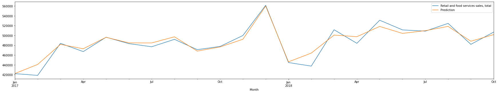

3.7.1.7.3. Compute the absolute difference between actual sales with forecasted sales

3.7.1.7.3。计算实际销售额与预期销售额之间的绝对差额

Retail_and_food_services_sales_total_validate['Abs Diff'] = (Retail_and_food_services_sales_total_validate['Retail and food services sales, total'] - Retail_and_food_services_sales_total_validate['Prediction']).abs()
Retail_and_food_services_sales_total_validate['Abs Diff %'] = (Retail_and_food_services_sales_total_validate['Retail and food services sales, total'] - Retail_and_food_services_sales_total_validate['Prediction']).abs()/Retail_and_food_services_sales_total_validate['Retail and food services sales, total']
Retail_and_food_services_sales_total_validate.loc['Average Abs Diff %'] = pd.Series(Retail_and_food_services_sales_total_validate['Abs Diff %'].mean(), index = ['Abs Diff %'])
Retail_and_food_services_sales_total_validate.loc['Min Abs Diff %'] = pd.Series(Retail_and_food_services_sales_total_validate['Abs Diff %'].min(), index = ['Abs Diff %'])
Retail_and_food_services_sales_total_validate.loc['Max Abs Diff %'] = pd.Series(Retail_and_food_services_sales_total_validate['Abs Diff %'].max(), index = ['Abs Diff %'])
Retail_and_food_services_sales_total_validate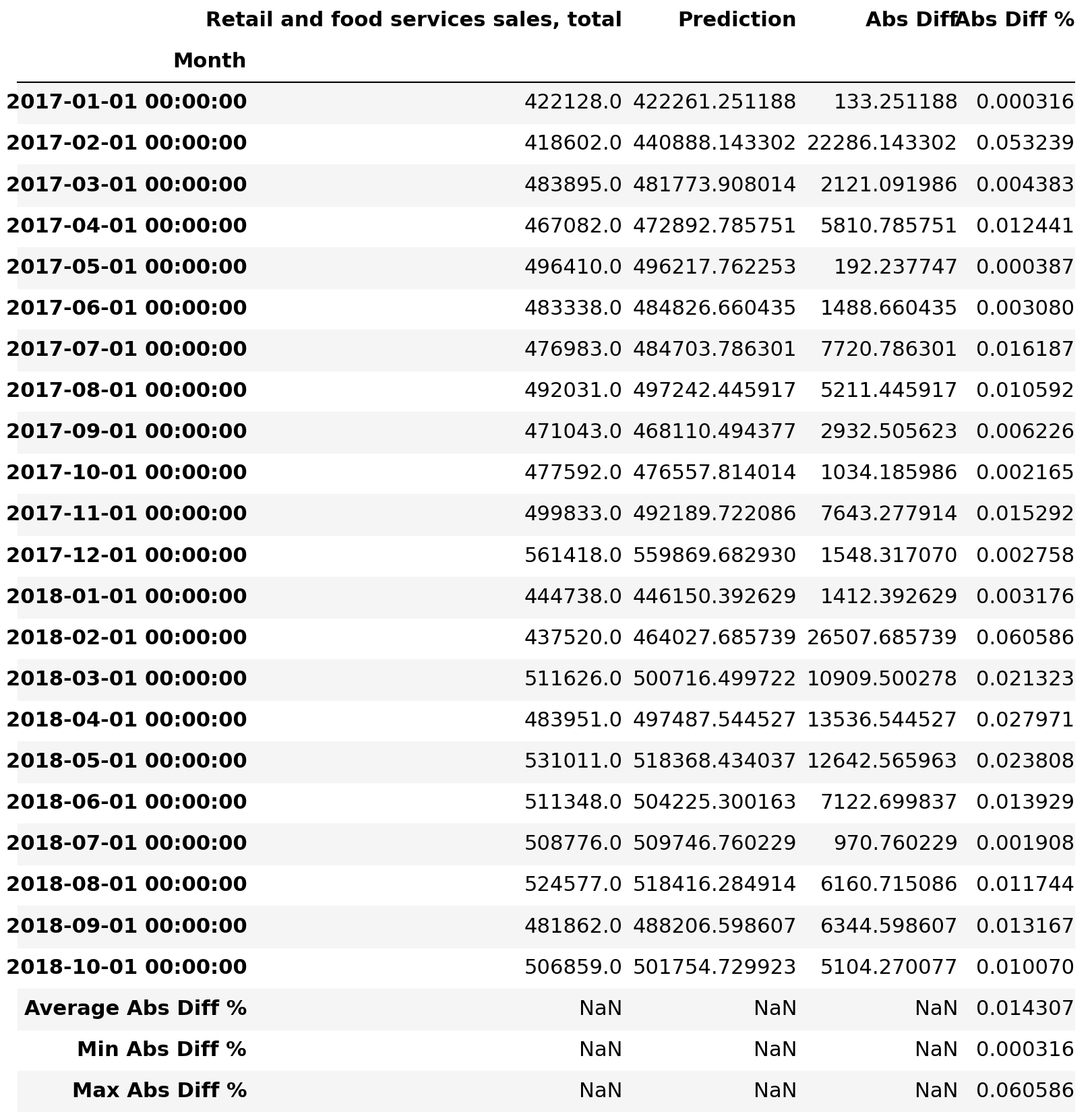

3.7.1.7.4. Compare all historical/actual sales data with forecast.

3.7.1.7.4。将所有历史/实际销售数据与预测进行比较。

Retail_and_food_services_sales_total = monthly_retail_data.filter(items=['Retail and food services sales, total'])
Retail_and_food_services_sales_total_1 = Retail_and_food_services_sales_total.loc['2005-01-01':'2016-12-01']
Retail_and_food_services_sales_total_2 = Retail_and_food_services_sales_total.loc['2017-01-01':]Retail_and_food_services_sales_total_forecast_all = Retail_and_food_services_sales_total_fit.predict(n_periods=48)
Retail_and_food_services_sales_total_forecast_allarray([422261.2511875 , 440888.14330158, 481773.90801362, 472892.78575083,
       496217.76225349, 484826.66043455, 484703.78630138, 497242.44591658,
       468110.4943768 , 476557.81401408, 492189.72208598, 559869.68293006,
       446150.39262897, 464027.68573856, 500716.49972167, 497487.54452719,
       518368.43403657, 504225.30016304, 509746.76022861, 518416.2849135 ,
       488206.59860748, 501754.72992269, 512491.23912928, 580833.12330101,
       471198.85797472, 483641.90137572, 522631.05496429, 522105.93519621,
       537541.53590709, 527082.60266315, 533700.49897643, 537430.90499257,
       511908.96278783, 524877.51821856, 531638.81672785, 605204.79125271,
       493406.95693487, 503194.82002935, 547436.60589097, 543404.29323055,
       557727.68441618, 552050.62025052, 554180.32437165, 558413.02423225,
       536758.59750276, 544705.71595078, 553500.48736504, 629672.63189599])Retail_and_food_services_sales_total_validate_all = pd.DataFrame(Retail_and_food_services_sales_total_forecast_all, index = Retail_and_food_services_sales_total_2.index, columns=['Prediction'])
Retail_and_food_services_sales_total_validate_all = pd.concat([Retail_and_food_services_sales_total_2, Retail_and_food_services_sales_total_validate_all], axis=1)
Retail_and_food_services_sales_total_validate_all = Retail_and_food_services_sales_total_1.append(Retail_and_food_services_sales_total_validate_all, sort=True)Retail_and_food_services_sales_total_validate_all.plot()
plt.pyplot.show()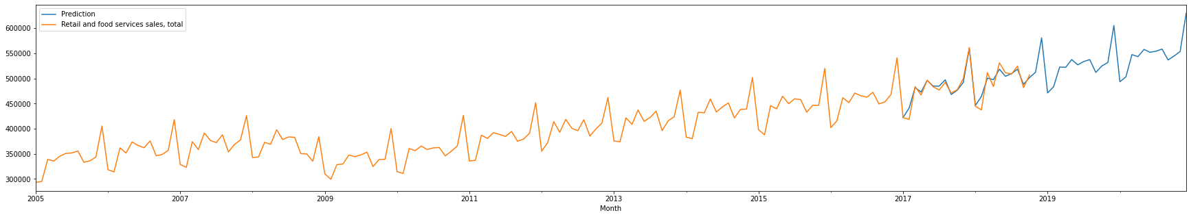

3.7.2. Retail sales and food services excl motor vehicle and parts

3.7.2。零售和食品服务，不包括机动车和零件

3.7.2.1. Filter Monthly Retail Data to just Retail sales and food services excl motor vehicle and parts data

3.7.2.1。将每月零售数据过滤为仅零售和食品服务(不包括机动车和零件数据)

Retail_sales_and_food_services_excl_motor_vehicle_and_parts_data = monthly_retail_actuals.filter(items=['Retail sales and food services excl motor vehicle and parts'])print('All: ', Retail_sales_and_food_services_excl_motor_vehicle_and_parts_data.shape)All:  (166, 1)

3.7.2.2. Split the data into Train and Test data

3.7.2.2。将数据分为训练和测试数据

We will be diving data into two sets of data:

我们将把数据分为两组数据：

Train Data
火车数据
Test Data
测试数据

通常我们使用70 Train / 30 Test(70/30)split，80 Train / 20 Test(80/20)split，90 Train / 10 Test(90/10)split甚至是95 Train / 5 Test(95/5)火车数据用于创建预测，测试数据用于验证预测。为简化起见，我们将数据拆分如下：

Train Data: January 2005 thru December 2016
火车数据：2005年1月至2016年12月
Test Data: January 2017 thru October 2018
测试数据：2017年1月至2018年10月

Retail_sales_and_food_services_excl_motor_vehicle_and_parts_train = Retail_sales_and_food_services_excl_motor_vehicle_and_parts_data.loc['2005-01-01':'2016-12-01']
Retail_sales_and_food_services_excl_motor_vehicle_and_parts_test = Retail_sales_and_food_services_excl_motor_vehicle_and_parts_data.loc['2017-01-01':]

3.7.2.3. Validate data split was done correctly

3.7.2.3。验证数据分割是否正确完成

print( 'Train: ', Retail_sales_and_food_services_excl_motor_vehicle_and_parts_train.shape)
print( 'Test: ', Retail_sales_and_food_services_excl_motor_vehicle_and_parts_test.shape)Train:  (144, 1)
Test:  (22, 1)

3.7.2.4. Train Forecast Model for Retail and food services sales, total using ARIMA (Autoregressive Integrated Moving Average) Model to find optimal Hyper-Parameters

3.7.2.4。训练零售和食品服务销售的预测模型，使用ARIMA(自回归综合移动平均线)模型进行总预测以找到最佳的超参数

ARIMA Model is bit difficult to explain, but it is best way to create a forecast of times series data. If you want to know more, here goes:

ARIMA模型有点难以解释，但它是创建时间序列数据预测的最佳方法。如果您想了解更多，这里有：

AR: Autoregression. A model that uses the dependent relationship between an observation and some number of lagged observations.
AR：自回归。一种模型，它使用观察值和一些滞后观察值之间的依赖关系。
I: Integrated. The use of differencing of raw observations (e.g. subtracting an observation from an observation at the previous time step) in order to make the time series stationary.
一：集成。为了使时间序列固定，使用原始观测值的差异(例如，从上一个时间步长的观测值中减去观测值)。
MA: Moving Average. A model that uses the dependency between an observation and a residual error from a moving average model applied to lagged observations.
MA：移动平均线。一种模型，该模型使用观察值与应用于滞后观察值的移动平均模型的残差之间的依赖关系。

3.7.2.4.1. Find the best fit using brute force search using train data

3.7.2.4.1。通过使用火车数据的蛮力搜索找到最合适的

Please note the parameters used:

请注意使用的参数：

m=12 (Denotes that retail sales data is monthly)
m = 12(表示每月零售数据)
seasonal=True (Denotes that retail sales data has seasonality)
Seasons = True(表示零售数据具有季节性)
stepwise=False (Denotes brute force search since dataset is small, not intelligent search)
stepwise = False(由于数据集很小而不是智能搜索，因此表示蛮力搜索)
d = 1 (Denotes that data is not stationary and differencing of data is needed, despite ADF test. KPSS test recommends d=’1')
d = 1(表示尽管ADF测试，数据仍不稳定，并且需要对数据进行区分。KPSS测试建议d ='1')

Retail_sales_and_food_services_excl_motor_vehicle_and_parts_fit = pm.auto_arima(Retail_sales_and_food_services_excl_motor_vehicle_and_parts_train, 
                           m=12,
                           seasonal=True,
                           d=1,
                           trace=True,
                           error_action='ignore',  
                           suppress_warnings=True, 
                           stepwise=False)ARIMA(0,1,0)(0,1,0)[12]             : AIC=2677.581, Time=0.05 sec
 ARIMA(0,1,0)(0,1,1)[12]             : AIC=2682.947, Time=0.26 sec
 ARIMA(0,1,0)(0,1,2)[12]             : AIC=2679.448, Time=0.68 sec
 ARIMA(0,1,0)(1,1,0)[12]             : AIC=2679.619, Time=0.14 sec
 ARIMA(0,1,0)(1,1,1)[12]             : AIC=2686.764, Time=0.46 sec
 ARIMA(0,1,0)(1,1,2)[12]             : AIC=2678.702, Time=1.28 sec
 ARIMA(0,1,0)(2,1,0)[12]             : AIC=2679.356, Time=0.54 sec
 ARIMA(0,1,0)(2,1,1)[12]             : AIC=2687.080, Time=1.45 sec
 ARIMA(0,1,0)(2,1,2)[12]             : AIC=2676.032, Time=5.00 sec
 ARIMA(0,1,1)(0,1,0)[12]             : AIC=2679.691, Time=0.07 sec
 ARIMA(0,1,1)(0,1,1)[12]             : AIC=2681.584, Time=0.40 sec
 ARIMA(0,1,1)(0,1,2)[12]             : AIC=2681.303, Time=1.07 sec
 ARIMA(0,1,1)(1,1,0)[12]             : AIC=2681.590, Time=0.26 sec
 ARIMA(0,1,1)(1,1,1)[12]             : AIC=2682.315, Time=0.66 sec
 ARIMA(0,1,1)(1,1,2)[12]             : AIC=2680.492, Time=1.94 sec
 ARIMA(0,1,1)(2,1,0)[12]             : AIC=2681.349, Time=0.83 sec
 ARIMA(0,1,1)(2,1,1)[12]             : AIC=2680.018, Time=2.45 sec
 ARIMA(0,1,1)(2,1,2)[12]             : AIC=2676.934, Time=5.62 sec
 ARIMA(0,1,2)(0,1,0)[12]             : AIC=2681.156, Time=0.09 sec
 ARIMA(0,1,2)(0,1,1)[12]             : AIC=2683.096, Time=0.50 sec
 ARIMA(0,1,2)(0,1,2)[12]             : AIC=2682.814, Time=1.14 sec
 ARIMA(0,1,2)(1,1,0)[12]             : AIC=2683.100, Time=0.35 sec
 ARIMA(0,1,2)(1,1,1)[12]             : AIC=2683.610, Time=0.92 sec
 ARIMA(0,1,2)(1,1,2)[12]             : AIC=2682.048, Time=2.11 sec
 ARIMA(0,1,2)(2,1,0)[12]             : AIC=2682.893, Time=0.96 sec
 ARIMA(0,1,2)(2,1,1)[12]             : AIC=2681.606, Time=3.34 sec
 ARIMA(0,1,3)(0,1,0)[12]             : AIC=2681.536, Time=0.14 sec
 ARIMA(0,1,3)(0,1,1)[12]             : AIC=2683.495, Time=0.73 sec
 ARIMA(0,1,3)(0,1,2)[12]             : AIC=2683.384, Time=1.60 sec
 ARIMA(0,1,3)(1,1,0)[12]             : AIC=2683.498, Time=0.42 sec
 ARIMA(0,1,3)(1,1,1)[12]             : AIC=2684.007, Time=1.49 sec
 ARIMA(0,1,3)(2,1,0)[12]             : AIC=2683.464, Time=1.20 sec
 ARIMA(0,1,4)(0,1,0)[12]             : AIC=2680.835, Time=0.20 sec
 ARIMA(0,1,4)(0,1,1)[12]             : AIC=2682.811, Time=0.71 sec
 ARIMA(0,1,4)(1,1,0)[12]             : AIC=2682.813, Time=0.51 sec
 ARIMA(0,1,5)(0,1,0)[12]             : AIC=2682.754, Time=0.28 sec
 ARIMA(1,1,0)(0,1,0)[12]             : AIC=2679.939, Time=0.06 sec
 ARIMA(1,1,0)(0,1,1)[12]             : AIC=2681.829, Time=0.34 sec
 ARIMA(1,1,0)(0,1,2)[12]             : AIC=2681.492, Time=0.92 sec
 ARIMA(1,1,0)(1,1,0)[12]             : AIC=2681.836, Time=0.26 sec
 ARIMA(1,1,0)(1,1,1)[12]             : AIC=2682.530, Time=0.61 sec
 ARIMA(1,1,0)(1,1,2)[12]             : AIC=2680.611, Time=1.76 sec
 ARIMA(1,1,0)(2,1,0)[12]             : AIC=2681.538, Time=0.86 sec
 ARIMA(1,1,0)(2,1,1)[12]             : AIC=2680.125, Time=1.47 sec
 ARIMA(1,1,0)(2,1,2)[12]             : AIC=2676.906, Time=4.70 sec
 ARIMA(1,1,1)(0,1,0)[12]             : AIC=2681.723, Time=0.44 sec
 ARIMA(1,1,1)(0,1,1)[12]             : AIC=2683.626, Time=1.51 sec
 ARIMA(1,1,1)(0,1,2)[12]             : AIC=2683.298, Time=3.45 sec
 ARIMA(1,1,1)(1,1,0)[12]             : AIC=2683.631, Time=1.19 sec
 ARIMA(1,1,1)(1,1,1)[12]             : AIC=2684.283, Time=2.30 sec
 ARIMA(1,1,1)(1,1,2)[12]             : AIC=2682.449, Time=5.46 sec
 ARIMA(1,1,1)(2,1,0)[12]             : AIC=2683.353, Time=3.24 sec
 ARIMA(1,1,1)(2,1,1)[12]             : AIC=2681.974, Time=4.81 sec
 ARIMA(1,1,2)(0,1,0)[12]             : AIC=2681.090, Time=0.58 sec
 ARIMA(1,1,2)(0,1,1)[12]             : AIC=2682.832, Time=1.68 sec
 ARIMA(1,1,2)(0,1,2)[12]             : AIC=2682.709, Time=2.61 sec
 ARIMA(1,1,2)(1,1,0)[12]             : AIC=2682.848, Time=1.39 sec
 ARIMA(1,1,2)(1,1,1)[12]             : AIC=2683.402, Time=1.54 sec
 ARIMA(1,1,2)(2,1,0)[12]             : AIC=2682.750, Time=4.39 sec
 ARIMA(1,1,3)(0,1,0)[12]             : AIC=2682.336, Time=0.69 sec
 ARIMA(1,1,3)(0,1,1)[12]             : AIC=2684.302, Time=1.39 sec
 ARIMA(1,1,3)(1,1,0)[12]             : AIC=2684.304, Time=0.91 sec
 ARIMA(1,1,4)(0,1,0)[12]             : AIC=2682.733, Time=0.78 sec
 ARIMA(2,1,0)(0,1,0)[12]             : AIC=2681.723, Time=0.12 sec
 ARIMA(2,1,0)(0,1,1)[12]             : AIC=2683.659, Time=0.39 sec
 ARIMA(2,1,0)(0,1,2)[12]             : AIC=2683.222, Time=1.12 sec
 ARIMA(2,1,0)(1,1,0)[12]             : AIC=2683.663, Time=0.38 sec
 ARIMA(2,1,0)(1,1,1)[12]             : AIC=2684.080, Time=1.06 sec
 ARIMA(2,1,0)(1,1,2)[12]             : AIC=2682.270, Time=2.05 sec
 ARIMA(2,1,0)(2,1,0)[12]             : AIC=2683.305, Time=1.13 sec
 ARIMA(2,1,0)(2,1,1)[12]             : AIC=2681.796, Time=3.38 sec
 ARIMA(2,1,1)(0,1,0)[12]             : AIC=2682.959, Time=0.60 sec
 ARIMA(2,1,1)(0,1,1)[12]             : AIC=2684.921, Time=1.51 sec
 ARIMA(2,1,1)(0,1,2)[12]             : AIC=2684.255, Time=3.22 sec
 ARIMA(2,1,1)(1,1,0)[12]             : AIC=2684.767, Time=1.70 sec
 ARIMA(2,1,1)(1,1,1)[12]             : AIC=2684.995, Time=2.64 sec
 ARIMA(2,1,1)(2,1,0)[12]             : AIC=2684.362, Time=5.70 sec
 ARIMA(2,1,2)(0,1,0)[12]             : AIC=2636.585, Time=0.73 sec
 ARIMA(2,1,2)(0,1,1)[12]             : AIC=2637.880, Time=3.05 sec
 ARIMA(2,1,2)(1,1,0)[12]             : AIC=2637.928, Time=2.98 sec
 ARIMA(2,1,3)(0,1,0)[12]             : AIC=2637.218, Time=1.37 sec
 ARIMA(3,1,0)(0,1,0)[12]             : AIC=2683.477, Time=0.22 sec
 ARIMA(3,1,0)(0,1,1)[12]             : AIC=2685.429, Time=0.51 sec
 ARIMA(3,1,0)(0,1,2)[12]             : AIC=2685.006, Time=1.35 sec
 ARIMA(3,1,0)(1,1,0)[12]             : AIC=2685.432, Time=0.54 sec
 ARIMA(3,1,0)(1,1,1)[12]             : AIC=2685.741, Time=1.22 sec
 ARIMA(3,1,0)(2,1,0)[12]             : AIC=2685.095, Time=1.29 sec
 ARIMA(3,1,1)(0,1,0)[12]             : AIC=2683.436, Time=0.64 sec
 ARIMA(3,1,1)(0,1,1)[12]             : AIC=2685.406, Time=1.93 sec
 ARIMA(3,1,1)(1,1,0)[12]             : AIC=2685.408, Time=1.47 sec
 ARIMA(3,1,2)(0,1,0)[12]             : AIC=2637.184, Time=0.96 sec
 ARIMA(4,1,0)(0,1,0)[12]             : AIC=2682.310, Time=0.21 sec
 ARIMA(4,1,0)(0,1,1)[12]             : AIC=2684.289, Time=0.66 sec
 ARIMA(4,1,0)(1,1,0)[12]             : AIC=2684.290, Time=0.78 sec
 ARIMA(4,1,1)(0,1,0)[12]             : AIC=2683.941, Time=0.67 sec
 ARIMA(5,1,0)(0,1,0)[12]             : AIC=2683.698, Time=0.32 sec
Total fit time: 135.175 seconds

3.7.2.4.2. View the summary of selected optimal hyper-parameters

3.7.2.4.2。查看所选最佳超参数的摘要

Retail_sales_and_food_services_excl_motor_vehicle_and_parts_fit.summary()

SARIMAX Results Dep. Variable: y No. Observations: 144 Model: SARIMAX(2, 1, 2)x(0, 1, [], 12) Log Likelihood -1313.293 Date: Sat, 15 Aug 2020 AIC 2636.585 Time: 15:10:34 BIC 2650.961 Sample: 0 HQIC 2642.427–144 Covariance Type: opg coef std err z P>|z| [0.025 0.975] ar.L1 -1.1736 0.009 -123.570 0.000 -1.192 -1.155 ar.L2 -0.9955 0.011 -94.464 0.000 -1.016 -0.975 ma.L1 1.1629 0.020 58.311 0.000 1.124 1.202 ma.L2 0.9919 0.030 32.824 0.000 0.933 1.051 sigma2 3.58e+07 6.1e-11 5.87e+17 0.000 3.58e+07 3.58e+07 Ljung-Box (Q): 64.78 Jarque-Bera (JB): 10.62 Prob(Q): 0.01 Prob(JB): 0.00 Heteroskedasticity (H): 0.68 Skew: -0.36 Prob(H) (two-sided): 0.20 Kurtosis: 4.20 Warnings:[1] Covariance matrix calculated using the outer product of gradients (complex-step).[2] Covariance matrix is singular or near-singular, with condition number 3.96e+33. Standard errors may be unstable.

SARIMAX结果部变量：y号。观察值：144模型：SARIMAX(2，1，2)x(0，1，[]，12)对数似然-1313.293日期：星期六，2020年8月15日AIC 2636.585时间：15:10:34 BIC 2650.961样本：0 HQIC 2642.427–144协方差类型：opg coef std err z P> | z | [0.025 0.975] ar.L1 -1.1736 0.009 -123.570 0.000 -1.192 -1.155 ar.L2 -0.9955 0.011 -94.464 0.000 -1.016 -0.975 ma.L1 1.1629 0.020 58.311 0.000 1.124 1.202 ma.L2 0.9919 0.030 32.824 0.000 0.933 1.051 sigma2 3.58 e + 07 6.1e-11 5.87e + 17 0.000 3.58e + 07 3.58e + 07 Ljung-Box(Q)：64.78 Jarque-Bera(JB)：10.62 Prob(Q)：0.01 Prob(JB)：0.00异方差( H)：0.68斜度：-0.36 Prob(H)(两侧)：0.20峰度：4.20警告：[1]使用梯度的外部乘积(复杂步骤)计算的协方差矩阵。[2] 协方差矩阵是奇异的或接近奇异的，条件编号为3.96e + 33。标准错误可能不稳定。

3.7.2.5. Fit Forecast Model

3.7.2.5。拟合预测模型

Retail_sales_and_food_services_excl_motor_vehicle_and_parts_fit.fit(Retail_sales_and_food_services_excl_motor_vehicle_and_parts_train)ARIMA(maxiter=50, method='lbfgs', order=(2, 1, 2), out_of_sample_size=0,
      scoring='mse', scoring_args={}, seasonal_order=(0, 1, 0, 12),
      start_params=None, suppress_warnings=True, trend=None,
      with_intercept=False)

3.7.2.6. Predict Forecast

3.7.2.6。预测预报

Retail_sales_and_food_services_excl_motor_vehicle_and_parts_forecast = Retail_sales_and_food_services_excl_motor_vehicle_and_parts_fit.predict(n_periods=22)Retail_sales_and_food_services_excl_motor_vehicle_and_parts_forecastarray([334487.17235321, 342747.07437798, 374081.16449735, 368048.44774989,
       389310.63822036, 379649.06267319, 377296.94794332, 385011.21131362,
       365651.84912897, 375604.9047198 , 393879.3474046 , 451940.38286472,
       349864.65950737, 357795.9522606 , 385688.95103369, 384021.98397148,
       403585.89752435, 391571.44341517, 393671.39048687, 398502.77357306,
       378094.91502015, 392148.40878545])

3.7.2.7. Validate Forecast

3.7.2.7。验证预测

3.7.2.7.1. Compare historical/actual sales data with forecast.

3.7.2.7.1。将历史/实际销售数据与预测进行比较。

Retail_sales_and_food_services_excl_motor_vehicle_and_parts_validate = pd.DataFrame(Retail_sales_and_food_services_excl_motor_vehicle_and_parts_forecast, index = Retail_sales_and_food_services_excl_motor_vehicle_and_parts_test.index, columns=['Prediction'])
Retail_sales_and_food_services_excl_motor_vehicle_and_parts_validate = pd.concat([Retail_sales_and_food_services_excl_motor_vehicle_and_parts_test, Retail_sales_and_food_services_excl_motor_vehicle_and_parts_validate], axis=1)
Retail_sales_and_food_services_excl_motor_vehicle_and_parts_validate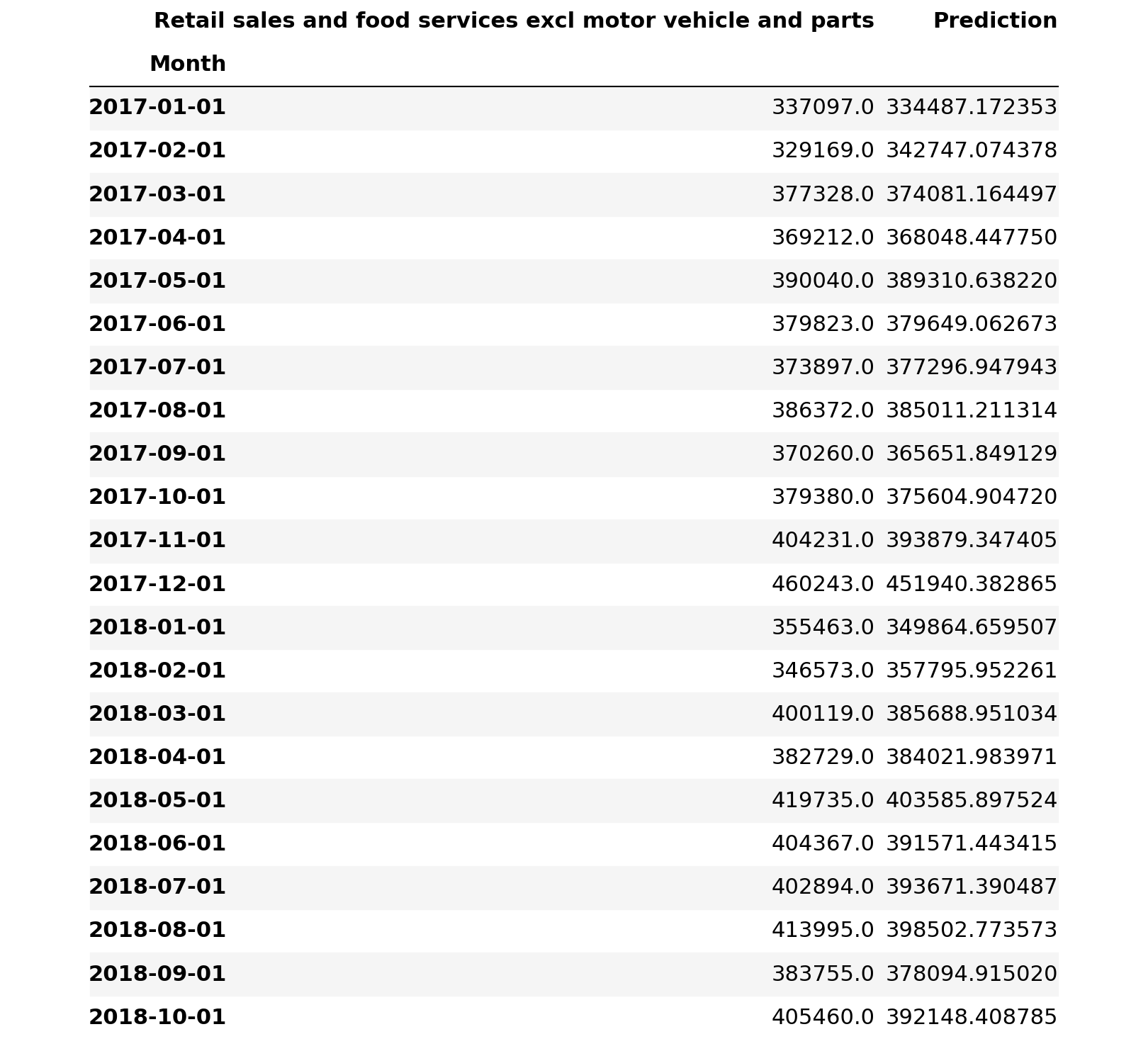

3.7.2.7.2. Plot the differences between historical/actual sales data with forecast

3.7.2.7.2。绘制历史/实际销售数据与预测之间的差异

Retail_sales_and_food_services_excl_motor_vehicle_and_parts_validate.plot()
plt.pyplot.show()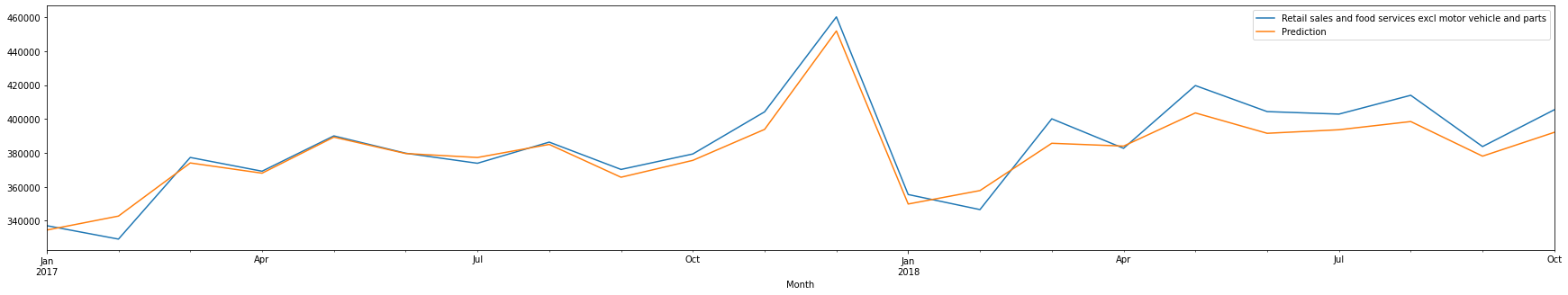

3.7.2.7.3. Compute the absolute difference between actual sales with forecasted sales

3.7.2.7.3。计算实际销售额与预期销售额之间的绝对差额

Retail_sales_and_food_services_excl_motor_vehicle_and_parts_validate['Abs Diff'] = (Retail_sales_and_food_services_excl_motor_vehicle_and_parts_validate['Retail sales and food services excl motor vehicle and parts'] - Retail_sales_and_food_services_excl_motor_vehicle_and_parts_validate['Prediction']).abs()
Retail_sales_and_food_services_excl_motor_vehicle_and_parts_validate['Abs Diff %'] = (Retail_sales_and_food_services_excl_motor_vehicle_and_parts_validate['Retail sales and food services excl motor vehicle and parts'] - Retail_sales_and_food_services_excl_motor_vehicle_and_parts_validate['Prediction']).abs()/Retail_sales_and_food_services_excl_motor_vehicle_and_parts_validate['Retail sales and food services excl motor vehicle and parts']
Retail_sales_and_food_services_excl_motor_vehicle_and_parts_validate.loc['Average Abs Diff %'] = pd.Series(Retail_sales_and_food_services_excl_motor_vehicle_and_parts_validate['Abs Diff %'].mean(), index = ['Abs Diff %'])
Retail_sales_and_food_services_excl_motor_vehicle_and_parts_validate.loc['Min Abs Diff %'] = pd.Series(Retail_sales_and_food_services_excl_motor_vehicle_and_parts_validate['Abs Diff %'].min(), index = ['Abs Diff %'])
Retail_sales_and_food_services_excl_motor_vehicle_and_parts_validate.loc['Max Abs Diff %'] = pd.Series(Retail_sales_and_food_services_excl_motor_vehicle_and_parts_validate['Abs Diff %'].max(), index = ['Abs Diff %'])
Retail_sales_and_food_services_excl_motor_vehicle_and_parts_validate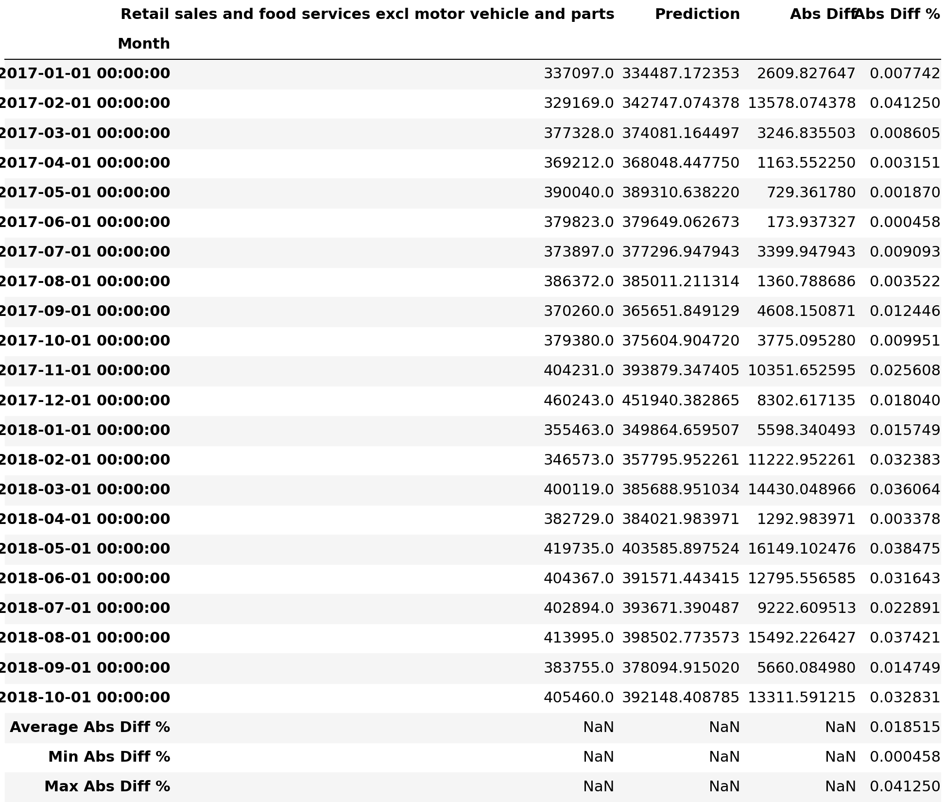

3.7.2.7.4. Compare all historical/actual sales data with forecast.

3.7.2.7.4。将所有历史/实际销售数据与预测进行比较。

Retail_sales_and_food_services_excl_motor_vehicle_and_parts = monthly_retail_data.filter(items=['Retail sales and food services excl motor vehicle and parts'])
Retail_sales_and_food_services_excl_motor_vehicle_and_parts_1 = Retail_sales_and_food_services_excl_motor_vehicle_and_parts.loc['2005-01-01':'2016-12-01']
Retail_sales_and_food_services_excl_motor_vehicle_and_parts_2 = Retail_sales_and_food_services_excl_motor_vehicle_and_parts.loc['2017-01-01':]Retail_sales_and_food_services_excl_motor_vehicle_and_parts_forecast_all = Retail_sales_and_food_services_excl_motor_vehicle_and_parts_fit.predict(n_periods=48)
Retail_sales_and_food_services_excl_motor_vehicle_and_parts_forecast_allarray([334487.17235321, 342747.07437798, 374081.16449735, 368048.44774989,
       389310.63822036, 379649.06267319, 377296.94794332, 385011.21131362,
       365651.84912897, 375604.9047198 , 393879.3474046 , 451940.38286472,
       349864.65950737, 357795.9522606 , 385688.95103369, 384021.98397148,
       403585.89752435, 391571.44341517, 393671.39048687, 398502.77357306,
       378094.91502015, 392148.40878545, 406654.15512668, 465056.36597596,
       366331.91803593, 369990.36377622, 399562.01536307, 400178.47505453,
       415391.37421162, 406210.34499792, 409316.24000579, 410146.35399121,
       393433.1588837 , 407133.64398028, 418375.70189631, 480959.74353686,
       380576.27174316, 382018.85889838, 415842.68336702, 413674.45975772,
       427922.60121176, 422645.97664357, 422129.88836982, 423324.1377132 ,
       409789.21995739, 419397.04012895, 432278.49849832, 497012.66603804])Retail_sales_and_food_services_excl_motor_vehicle_and_parts_validate_all = pd.DataFrame(Retail_sales_and_food_services_excl_motor_vehicle_and_parts_forecast_all, index = Retail_sales_and_food_services_excl_motor_vehicle_and_parts_2.index, columns=['Prediction'])
Retail_sales_and_food_services_excl_motor_vehicle_and_parts_validate_all = pd.concat([Retail_sales_and_food_services_excl_motor_vehicle_and_parts_2, Retail_sales_and_food_services_excl_motor_vehicle_and_parts_validate_all], axis=1)
Retail_sales_and_food_services_excl_motor_vehicle_and_parts_validate_all = Retail_sales_and_food_services_excl_motor_vehicle_and_parts_1.append(Retail_sales_and_food_services_excl_motor_vehicle_and_parts_validate_all, sort=True)Retail_and_food_services_sales_total_validate_all.plot()
plt.pyplot.show()

3.7.3. Retail sales and food services excl gasoline stations

3.7.3。零售和食品服务，不包括加油站

3.7.3.1. Filter Monthly Retail Data to just Retail sales and food services excl gasoline stations data

3.7.3.1。将每月零售数据过滤为零售和食品服务除外加油站数据

Retail_sales_and_food_services_excl_gasoline_stations_data = monthly_retail_actuals.filter(items=['Retail sales and food services excl gasoline stations'])print('All: ', Retail_sales_and_food_services_excl_gasoline_stations_data.shape)All:  (166, 1)

3.7.3.2. Split the data into Train and Test data

3.7.3.2。将数据分为训练和测试数据

We will be diving data into two sets of data:

我们将把数据分为两组数据：

Train Data
火车数据
Test Data
测试数据

Train Data: January 2005 thru December 2016
火车数据：2005年1月至2016年12月
Test Data: January 2017 thru October 2018
测试数据：2017年1月至2018年10月

Retail_sales_and_food_services_excl_gasoline_stations_train = Retail_sales_and_food_services_excl_gasoline_stations_data.loc['2005-01-01':'2016-12-01']
Retail_sales_and_food_services_excl_gasoline_stations_test = Retail_sales_and_food_services_excl_gasoline_stations_data.loc['2017-01-01':]

3.7.3.3. Validate data split was done correctly

3.7.3.3。验证数据分割是否正确完成

print( 'Train: ', Retail_sales_and_food_services_excl_gasoline_stations_train.shape)
print( 'Test: ', Retail_sales_and_food_services_excl_gasoline_stations_test.shape)Train:  (144, 1)
Test:  (22, 1)

3.7.3.4. Train Forecast Model for Retail and food services sales, total using ARIMA (Autoregressive Integrated Moving Average) Model to find optimal Hyper-Parameters

3.7.3.4。训练零售和食品服务销售的预测模型，使用ARIMA(自回归综合移动平均线)模型进行总预测以找到最佳的超参数

ARIMA Model is bit difficult to explain, but it is best way to create a forecast of times series data. If you want to know more, here goes:

ARIMA模型有点难以解释，但它是创建时间序列数据预测的最佳方法。如果您想了解更多，这里有：

AR: Autoregression. A model that uses the dependent relationship between an observation and some number of lagged observations.
AR：自回归。一种模型，它使用观察值和一些滞后观察值之间的依赖关系。
I: Integrated. The use of differencing of raw observations (e.g. subtracting an observation from an observation at the previous time step) in order to make the time series stationary.
一：集成。 The use of differencing of raw observations (eg subtracting an observation from an observation at the previous time step) in order to make the time series stationary.
MA: Moving Average. A model that uses the dependency between an observation and a residual error from a moving average model applied to lagged observations.
MA: Moving Average. A model that uses the dependency between an observation and a residual error from a moving average model applied to lagged observations.

3.7.3.4.1. Find the best fit using brute force search using train data

Please note the parameters used:

m=12 (Denote that retail sales data is monthly)
m=12 (Denote that retail sales data is monthly)
seasonal=True (Denotes that retail sales data has seasonality)
seasonal=True (Denotes that retail sales data has seasonality)
d=1 (Denotes that retail sales data is not stationary and differencing of 1 is required as noted on section 3.5.9.3)
d=1 (Denotes that retail sales data is not stationary and differencing of 1 is required as noted on section 3.5.9.3)
stepwise=False (Denotes brute force search since dataset is small, not intelligent search)
stepwise=False (Denotes brute force search since dataset is small, not intelligent search)

Retail_sales_and_food_services_excl_gasoline_stations_fit = pm.auto_arima(Retail_sales_and_food_services_excl_gasoline_stations_train, 
                           m=12,
                           seasonal=True,
                           d=1,
                           trace=True,
                           error_action='ignore',  
                           suppress_warnings=True, 
                           stepwise=False)ARIMA(0,1,0)(0,1,0)[12]             : AIC=2731.193, Time=0.06 sec
 ARIMA(0,1,0)(0,1,1)[12]             : AIC=2733.200, Time=0.35 sec
 ARIMA(0,1,0)(0,1,2)[12]             : AIC=2734.033, Time=0.74 sec
 ARIMA(0,1,0)(1,1,0)[12]             : AIC=2732.907, Time=0.14 sec
 ARIMA(0,1,0)(1,1,1)[12]             : AIC=2733.673, Time=0.44 sec
 ARIMA(0,1,0)(1,1,2)[12]             : AIC=2733.573, Time=1.41 sec
 ARIMA(0,1,0)(2,1,0)[12]             : AIC=2733.075, Time=0.58 sec
 ARIMA(0,1,0)(2,1,1)[12]             : AIC=2733.310, Time=1.20 sec
 ARIMA(0,1,0)(2,1,2)[12]             : AIC=2729.364, Time=4.79 sec
 ARIMA(0,1,1)(0,1,0)[12]             : AIC=2736.626, Time=0.08 sec
 ARIMA(0,1,1)(0,1,1)[12]             : AIC=2738.625, Time=0.35 sec
 ARIMA(0,1,1)(0,1,2)[12]             : AIC=2738.112, Time=0.97 sec
 ARIMA(0,1,1)(1,1,0)[12]             : AIC=2738.625, Time=0.28 sec
 ARIMA(0,1,1)(1,1,1)[12]             : AIC=2738.254, Time=0.70 sec
 ARIMA(0,1,1)(1,1,2)[12]             : AIC=2736.608, Time=1.81 sec
 ARIMA(0,1,1)(2,1,0)[12]             : AIC=2738.323, Time=0.94 sec
 ARIMA(0,1,1)(2,1,1)[12]             : AIC=2736.092, Time=1.34 sec
 ARIMA(0,1,1)(2,1,2)[12]             : AIC=2732.761, Time=6.70 sec
 ARIMA(0,1,2)(0,1,0)[12]             : AIC=2738.053, Time=0.10 sec
 ARIMA(0,1,2)(0,1,1)[12]             : AIC=2740.047, Time=0.42 sec
 ARIMA(0,1,2)(0,1,2)[12]             : AIC=2739.515, Time=1.15 sec
 ARIMA(0,1,2)(1,1,0)[12]             : AIC=2740.047, Time=0.42 sec
 ARIMA(0,1,2)(1,1,1)[12]             : AIC=2739.364, Time=1.56 sec
 ARIMA(0,1,2)(1,1,2)[12]             : AIC=2737.925, Time=2.24 sec
 ARIMA(0,1,2)(2,1,0)[12]             : AIC=2739.770, Time=1.02 sec
 ARIMA(0,1,2)(2,1,1)[12]             : AIC=2737.435, Time=2.03 sec
 ARIMA(0,1,3)(0,1,0)[12]             : AIC=2736.253, Time=0.15 sec
 ARIMA(0,1,3)(0,1,1)[12]             : AIC=2738.225, Time=0.58 sec
 ARIMA(0,1,3)(0,1,2)[12]             : AIC=2738.019, Time=1.61 sec
 ARIMA(0,1,3)(1,1,0)[12]             : AIC=2738.227, Time=0.42 sec
 ARIMA(0,1,3)(1,1,1)[12]             : AIC=2737.620, Time=1.32 sec
 ARIMA(0,1,3)(2,1,0)[12]             : AIC=2738.264, Time=1.29 sec
 ARIMA(0,1,4)(0,1,0)[12]             : AIC=2734.090, Time=0.23 sec
 ARIMA(0,1,4)(0,1,1)[12]             : AIC=2736.026, Time=0.77 sec
 ARIMA(0,1,4)(1,1,0)[12]             : AIC=2736.030, Time=0.49 sec
 ARIMA(0,1,5)(0,1,0)[12]             : AIC=2730.982, Time=0.35 sec
 ARIMA(1,1,0)(0,1,0)[12]             : AIC=2737.232, Time=0.09 sec
 ARIMA(1,1,0)(0,1,1)[12]             : AIC=2739.231, Time=0.39 sec
 ARIMA(1,1,0)(0,1,2)[12]             : AIC=2738.681, Time=0.94 sec
 ARIMA(1,1,0)(1,1,0)[12]             : AIC=2739.231, Time=0.27 sec
 ARIMA(1,1,0)(1,1,1)[12]             : AIC=2738.834, Time=0.75 sec
 ARIMA(1,1,0)(1,1,2)[12]             : AIC=2737.124, Time=1.68 sec
 ARIMA(1,1,0)(2,1,0)[12]             : AIC=2738.894, Time=0.95 sec
 ARIMA(1,1,0)(2,1,1)[12]             : AIC=2736.599, Time=2.37 sec
 ARIMA(1,1,0)(2,1,2)[12]             : AIC=2733.087, Time=5.62 sec
 ARIMA(1,1,1)(0,1,0)[12]             : AIC=2733.379, Time=0.60 sec
 ARIMA(1,1,1)(0,1,1)[12]             : AIC=2741.805, Time=0.84 sec
 ARIMA(1,1,1)(0,1,2)[12]             : AIC=2741.191, Time=2.45 sec
 ARIMA(1,1,1)(1,1,0)[12]             : AIC=2741.805, Time=0.71 sec
 ARIMA(1,1,1)(1,1,1)[12]             : AIC=2741.268, Time=1.83 sec
 ARIMA(1,1,1)(1,1,2)[12]             : AIC=2739.543, Time=3.74 sec
 ARIMA(1,1,1)(2,1,0)[12]             : AIC=2741.421, Time=2.17 sec
 ARIMA(1,1,1)(2,1,1)[12]             : AIC=2739.014, Time=2.90 sec
 ARIMA(1,1,2)(0,1,0)[12]             : AIC=2736.829, Time=0.29 sec
 ARIMA(1,1,2)(0,1,1)[12]             : AIC=2738.795, Time=1.17 sec
 ARIMA(1,1,2)(0,1,2)[12]             : AIC=2738.364, Time=3.97 sec
 ARIMA(1,1,2)(1,1,0)[12]             : AIC=2738.797, Time=1.03 sec
 ARIMA(1,1,2)(1,1,1)[12]             : AIC=2737.930, Time=1.78 sec
 ARIMA(1,1,2)(2,1,0)[12]             : AIC=2738.639, Time=2.62 sec
 ARIMA(1,1,3)(0,1,0)[12]             : AIC=2737.316, Time=0.35 sec
 ARIMA(1,1,3)(0,1,1)[12]             : AIC=2739.274, Time=1.79 sec
 ARIMA(1,1,3)(1,1,0)[12]             : AIC=2739.276, Time=0.98 sec
 ARIMA(1,1,4)(0,1,0)[12]             : AIC=2737.341, Time=0.50 sec
 ARIMA(2,1,0)(0,1,0)[12]             : AIC=2745.253, Time=0.13 sec
 ARIMA(2,1,0)(0,1,1)[12]             : AIC=2747.244, Time=0.39 sec
 ARIMA(2,1,0)(0,1,2)[12]             : AIC=2746.303, Time=1.19 sec
 ARIMA(2,1,0)(1,1,0)[12]             : AIC=2747.245, Time=0.48 sec
 ARIMA(2,1,0)(1,1,1)[12]             : AIC=2746.125, Time=0.96 sec
 ARIMA(2,1,0)(1,1,2)[12]             : AIC=2744.144, Time=2.21 sec
 ARIMA(2,1,0)(2,1,0)[12]             : AIC=2746.602, Time=1.22 sec
 ARIMA(2,1,0)(2,1,1)[12]             : AIC=2743.573, Time=2.37 sec
 ARIMA(2,1,1)(0,1,0)[12]             : AIC=2743.967, Time=0.47 sec
 ARIMA(2,1,1)(0,1,1)[12]             : AIC=2745.909, Time=1.60 sec
 ARIMA(2,1,1)(0,1,2)[12]             : AIC=2745.105, Time=3.96 sec
 ARIMA(2,1,1)(1,1,0)[12]             : AIC=2745.913, Time=1.93 sec
 ARIMA(2,1,1)(1,1,1)[12]             : AIC=2744.526, Time=1.20 sec
 ARIMA(2,1,1)(2,1,0)[12]             : AIC=2745.438, Time=2.88 sec
 ARIMA(2,1,2)(0,1,0)[12]             : AIC=2673.693, Time=1.03 sec
 ARIMA(2,1,2)(0,1,1)[12]             : AIC=2674.937, Time=3.26 sec
 ARIMA(2,1,2)(1,1,0)[12]             : AIC=2675.184, Time=4.03 sec
 ARIMA(2,1,3)(0,1,0)[12]             : AIC=2675.348, Time=1.16 sec
 ARIMA(3,1,0)(0,1,0)[12]             : AIC=2744.989, Time=0.19 sec
 ARIMA(3,1,0)(0,1,1)[12]             : AIC=2746.958, Time=0.58 sec
 ARIMA(3,1,0)(0,1,2)[12]             : AIC=2746.326, Time=1.50 sec
 ARIMA(3,1,0)(1,1,0)[12]             : AIC=2746.960, Time=0.56 sec
 ARIMA(3,1,0)(1,1,1)[12]             : AIC=2745.893, Time=1.34 sec
 ARIMA(3,1,0)(2,1,0)[12]             : AIC=2746.613, Time=1.37 sec
 ARIMA(3,1,1)(0,1,0)[12]             : AIC=2742.687, Time=0.60 sec
 ARIMA(3,1,1)(0,1,1)[12]             : AIC=2744.618, Time=1.36 sec
 ARIMA(3,1,1)(1,1,0)[12]             : AIC=2744.622, Time=1.19 sec
 ARIMA(3,1,2)(0,1,0)[12]             : AIC=2675.021, Time=1.52 sec
 ARIMA(4,1,0)(0,1,0)[12]             : AIC=2742.172, Time=0.23 sec
 ARIMA(4,1,0)(0,1,1)[12]             : AIC=2744.068, Time=0.73 sec
 ARIMA(4,1,0)(1,1,0)[12]             : AIC=2744.074, Time=0.80 sec
 ARIMA(4,1,1)(0,1,0)[12]             : AIC=2743.127, Time=0.95 sec
 ARIMA(5,1,0)(0,1,0)[12]             : AIC=2740.445, Time=0.34 sec
Total fit time: 125.723 seconds

3.7.3.4.2. View the summary of selected optimal hyper-parameters

Retail_sales_and_food_services_excl_gasoline_stations_fit.summary()

SARIMAX Results Dep. Variable: y No. Observations: 144 Model: SARIMAX(2, 1, 2)x(0, 1, [], 12) Log Likelihood -1331.847 Date: Sat, 15 Aug 2020 AIC 2673.693 Time: 15:12:42 BIC 2688.069 Sample: 0 HQIC 2679.535–144 Covariance Type: opg coef std err z P>|z| [0.025 0.975] ar.L1 -1.1725 0.007 -180.210 0.000 -1.185 -1.160 ar.L2 -0.9947 0.007 -139.376 0.000 -1.009 -0.981 ma.L1 1.1601 0.018 65.947 0.000 1.126 1.195 ma.L2 0.9935 0.031 32.550 0.000 0.934 1.053 sigma2 4.156e+07 5.27e-11 7.88e+17 0.000 4.16e+07 4.16e+07 Ljung-Box (Q): 74.58 Jarque-Bera (JB): 1.93 Prob(Q): 0.00 Prob(JB): 0.38 Heteroskedasticity (H): 1.04 Skew: -0.17 Prob(H) (two-sided): 0.90 Kurtosis: 3.49 Warnings:[1] Covariance matrix calculated using the outer product of gradients (complex-step).[2] Covariance matrix is singular or near-singular, with condition number 9.08e+33. Standard errors may be unstable.

3.7.3.5. Fit Forecast Model

Retail_sales_and_food_services_excl_gasoline_stations_fit.fit(Retail_sales_and_food_services_excl_gasoline_stations_train)ARIMA(maxiter=50, method='lbfgs', order=(2, 1, 2), out_of_sample_size=0,
      scoring='mse', scoring_args={}, seasonal_order=(0, 1, 0, 12),
      start_params=None, suppress_warnings=True, trend=None,
      with_intercept=False)

3.7.3.6. Predict Forecast

Retail_sales_and_food_services_excl_gasoline_stations_forecast = Retail_sales_and_food_services_excl_gasoline_stations_fit.predict(n_periods=22)Retail_sales_and_food_services_excl_gasoline_stations_forecastarray([389347.90468944, 410090.65272841, 446513.78163093, 436026.29046246,
       456071.84586912, 443427.95208676, 443687.91311935, 457281.24550431,
       428878.49797163, 436455.763191  , 455160.19362191, 521486.50182765,
       410438.33799152, 430369.38945941, 462522.27230556, 457849.2338632 ,
       475324.58319701, 459910.86483611, 465975.11399183, 475517.7199756 ,
       446091.24166362, 458898.05726593])

3.7.3.7. Validate Forecast

3.7.3.7.1. Compare historical/actual sales data with forecast

Retail_sales_and_food_services_excl_gasoline_stations_validate = pd.DataFrame(Retail_sales_and_food_services_excl_gasoline_stations_forecast, index = Retail_sales_and_food_services_excl_gasoline_stations_test.index, columns=['Prediction'])
Retail_sales_and_food_services_excl_gasoline_stations_validate = pd.concat([Retail_sales_and_food_services_excl_gasoline_stations_test, Retail_sales_and_food_services_excl_gasoline_stations_validate], axis=1)
Retail_sales_and_food_services_excl_gasoline_stations_validate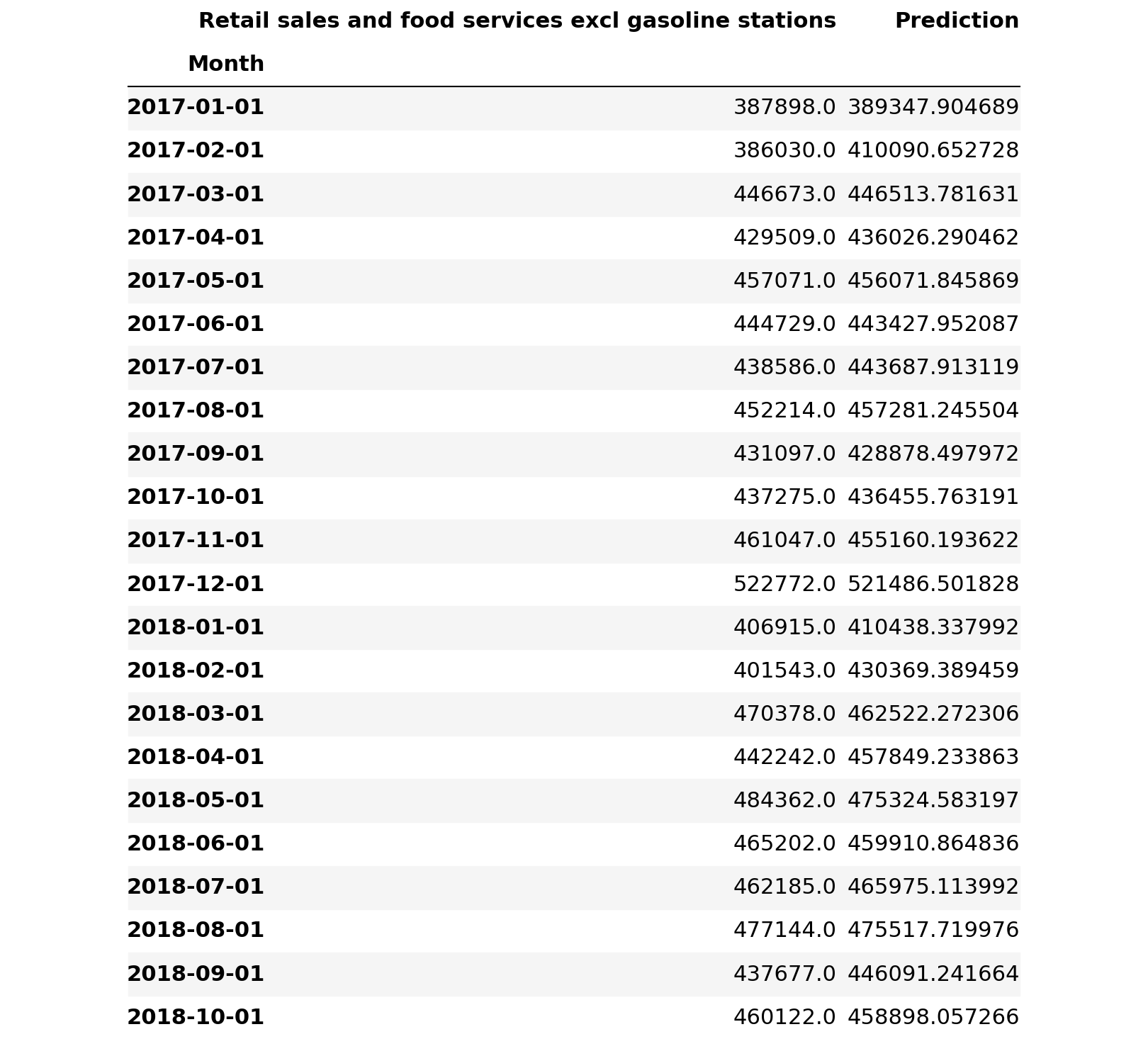

3.7.3.7.2. Plot the differences between historical/actual sales data with forecast.

Retail_sales_and_food_services_excl_gasoline_stations_validate.plot()
plt.pyplot.show()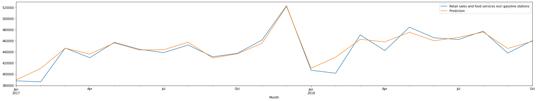

3.7.3.7.3. Compute the absolute difference between actual sales with forecasted sales

Retail_sales_and_food_services_excl_gasoline_stations_validate['Abs Diff'] = (Retail_sales_and_food_services_excl_gasoline_stations_validate['Retail sales and food services excl gasoline stations'] - Retail_sales_and_food_services_excl_gasoline_stations_validate['Prediction']).abs()
Retail_sales_and_food_services_excl_gasoline_stations_validate['Abs Diff %'] = (Retail_sales_and_food_services_excl_gasoline_stations_validate['Retail sales and food services excl gasoline stations'] - Retail_sales_and_food_services_excl_gasoline_stations_validate['Prediction']).abs()/Retail_sales_and_food_services_excl_gasoline_stations_validate['Retail sales and food services excl gasoline stations']
Retail_sales_and_food_services_excl_gasoline_stations_validate.loc['Average Abs Diff %'] = pd.Series(Retail_sales_and_food_services_excl_gasoline_stations_validate['Abs Diff %'].mean(), index = ['Abs Diff %'])
Retail_sales_and_food_services_excl_gasoline_stations_validate.loc['Min Abs Diff %'] = pd.Series(Retail_sales_and_food_services_excl_gasoline_stations_validate['Abs Diff %'].min(), index = ['Abs Diff %'])
Retail_sales_and_food_services_excl_gasoline_stations_validate.loc['Max Abs Diff %'] = pd.Series(Retail_sales_and_food_services_excl_gasoline_stations_validate['Abs Diff %'].max(), index = ['Abs Diff %'])
Retail_sales_and_food_services_excl_gasoline_stations_validate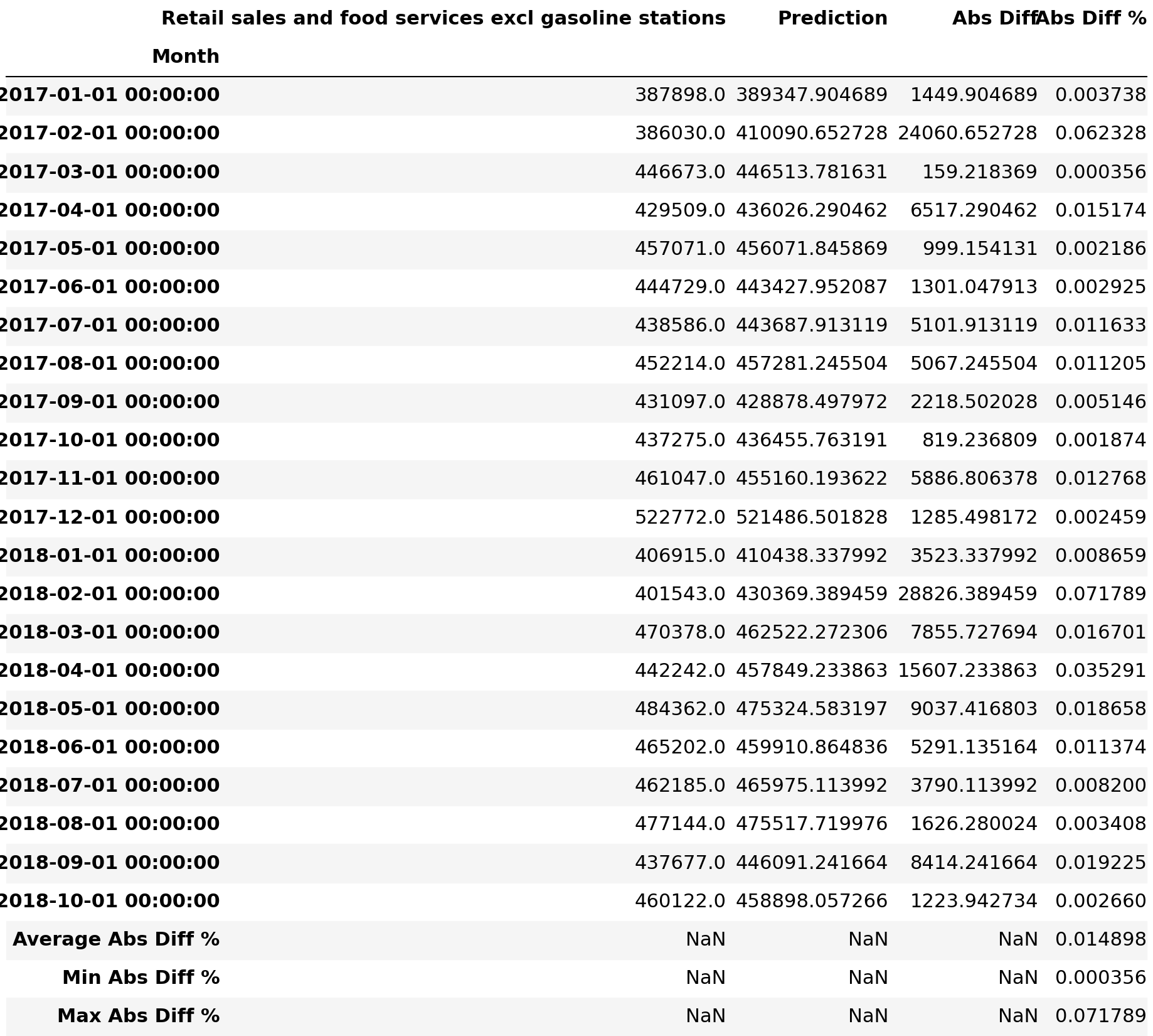

3.7.3.7.4. Compare all historical/actual sales data with forecast.

Retail_sales_and_food_services_excl_gasoline_stations = monthly_retail_data.filter(items=['Retail sales and food services excl gasoline stations'])
Retail_sales_and_food_services_excl_gasoline_stations_1 = Retail_sales_and_food_services_excl_gasoline_stations.loc['2005-01-01':'2016-12-01']
Retail_sales_and_food_services_excl_gasoline_stations_2 = Retail_sales_and_food_services_excl_gasoline_stations.loc['2017-01-01':]Retail_sales_and_food_services_excl_gasoline_stations_forecast_all = Retail_sales_and_food_services_excl_gasoline_stations_fit.predict(n_periods=48)
Retail_sales_and_food_services_excl_gasoline_stations_forecast_allarray([389347.90468944, 410090.65272841, 446513.78163093, 436026.29046246,
       456071.84586912, 443427.95208676, 443687.91311935, 457281.24550431,
       428878.49797163, 436455.763191  , 455160.19362191, 521486.50182765,
       410438.33799152, 430369.38945941, 462522.27230556, 457849.2338632 ,
       475324.58319701, 459910.86483611, 465975.11399183, 475517.7199756 ,
       446091.24166362, 458898.05726593, 472488.86560256, 539609.4207528 ,
       432716.37934562, 446985.32302152, 481644.29111252, 479664.72767169,
       491489.09222353, 480022.28789424, 487079.50523884, 491531.89155725,
       467086.26211044, 479115.92450276, 488663.63400115, 561297.94095416,
       451961.34143873, 463611.06064943, 503771.75662271, 497946.4347404 ,
       508807.68398572, 502295.47792655, 504501.17513945, 509713.97018704,
       489202.43264053, 495862.8146492 , 507793.10936635, 582974.43171978])Retail_sales_and_food_services_excl_gasoline_stations_validate_all = pd.DataFrame(Retail_sales_and_food_services_excl_gasoline_stations_forecast_all, index = Retail_sales_and_food_services_excl_gasoline_stations_2.index, columns=['Prediction'])
Retail_sales_and_food_services_excl_gasoline_stations_validate_all = pd.concat([Retail_sales_and_food_services_excl_gasoline_stations_2, Retail_sales_and_food_services_excl_gasoline_stations_validate_all], axis=1)
Retail_sales_and_food_services_excl_gasoline_stations_validate_all = Retail_sales_and_food_services_excl_gasoline_stations_1.append(Retail_sales_and_food_services_excl_gasoline_stations_validate_all, sort=True)Retail_sales_and_food_services_excl_gasoline_stations_validate_all.plot()
plt.pyplot.show()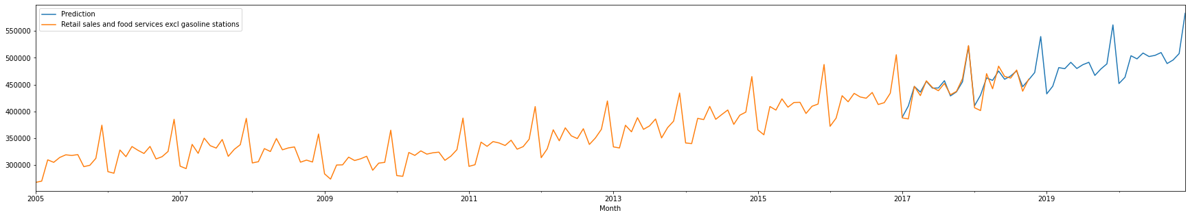

3.7.4. Retail sales and food services excl motor vehicle and parts and gasoline stations

3.7.4.1. Filter Monthly Retail Data to just Retail sales and food services excl motor vehicle and parts and gasoline stations data

Retail_sales_and_food_services_excl_motor_vehicle_and_parts_and_gasoline_stations_data = monthly_retail_actuals.filter(items=['Retail sales and food services excl motor vehicle and parts and gasoline stations'])print('All: ', Retail_sales_and_food_services_excl_motor_vehicle_and_parts_and_gasoline_stations_data.shape)All:  (166, 1)

3.7.4.2. Split the data into Train and Test data

We will be diving data into two sets of data:

Train Data
Train Data
Test Data
Test Data

Usually we use 70 Train/30 Test (70/30) split, 80 Train/20 Test (80/20) split, 90 Train/10 Test (90/10) split or even 95 Train/5 Test (95/5) where train data is used to create a forecast and test data is used to validate the forecast, but for simplification purposes, we will split the data as follows:

Train Data: January 2005 thru December 2016
Train Data: January 2005 thru December 2016
Test Data: January 2017 thru October 2018
Test Data: January 2017 thru October 2018

Retail_sales_and_food_services_excl_motor_vehicle_and_parts_and_gasoline_stations_train = Retail_sales_and_food_services_excl_motor_vehicle_and_parts_and_gasoline_stations_data.loc['2005-01-01':'2016-12-01']
Retail_sales_and_food_services_excl_motor_vehicle_and_parts_and_gasoline_stations_test = Retail_sales_and_food_services_excl_motor_vehicle_and_parts_and_gasoline_stations_data.loc['2017-01-01':]

3.7.4.3. Validate data split was done correctly

print( 'Train: ', Retail_sales_and_food_services_excl_motor_vehicle_and_parts_and_gasoline_stations_train.shape)
print( 'Test: ', Retail_sales_and_food_services_excl_motor_vehicle_and_parts_and_gasoline_stations_test.shape)Train:  (144, 1)
Test:  (22, 1)

3.7.4.4. Train Forecast Model for Retail and food services sales, total using ARIMA (Autoregressive Integrated Moving Average) Model to find optimal Hyper-Parameters

ARIMA Model is bit difficult to explain, but it is best way to create a forecast of times series data. If you want to know more, here goes:

AR: Autoregression. A model that uses the dependent relationship between an observation and some number of lagged observations.
AR: Autoregression. A model that uses the dependent relationship between an observation and some number of lagged observations.
I: Integrated. The use of differencing of raw observations (e.g. subtracting an observation from an observation at the previous time step) in order to make the time series stationary.
I: Integrated. The use of differencing of raw observations (eg subtracting an observation from an observation at the previous time step) in order to make the time series stationary.
MA: Moving Average. A model that uses the dependency between an observation and a residual error from a moving average model applied to lagged observations.
MA: Moving Average. A model that uses the dependency between an observation and a residual error from a moving average model applied to lagged observations.

3.7.4.4.1. Find the best fit using brute force search using train data

Please note the parameters used:

m=12 (Denote that retail sales data is monthly)
m=12 (Denote that retail sales data is monthly)
seasonal=True (Denotes that retail sales data has seasonality)
seasonal=True (Denotes that retail sales data has seasonality)
d=1 (Denotes that retail sales data is not stationary and differencing of 1 is required as noted on section 3.5.10.3)
d=1 (Denotes that retail sales data is not stationary and differencing of 1 is required as noted on section 3.5.10.3)
stepwise=False (Denotes brute force search since dataset is small, not intelligent search)
stepwise=False (Denotes brute force search since dataset is small, not intelligent search)

Retail_sales_and_food_services_excl_motor_vehicle_and_parts_and_gasoline_stations_fit = pm.auto_arima(Retail_sales_and_food_services_excl_motor_vehicle_and_parts_and_gasoline_stations_train, 
                           m=12,
                           seasonal=True,
                           d=1, 
                           trace=True,
                           error_action='ignore',  
                           suppress_warnings=True, 
                           stepwise=False)ARIMA(0,1,0)(0,1,0)[12]             : AIC=2631.176, Time=0.04 sec
 ARIMA(0,1,0)(0,1,1)[12]             : AIC=2633.371, Time=0.23 sec
 ARIMA(0,1,0)(0,1,2)[12]             : AIC=2634.663, Time=0.70 sec
 ARIMA(0,1,0)(1,1,0)[12]             : AIC=2633.424, Time=0.14 sec
 ARIMA(0,1,0)(1,1,1)[12]             : AIC=2634.672, Time=0.80 sec
 ARIMA(0,1,0)(1,1,2)[12]             : AIC=2634.120, Time=1.39 sec
 ARIMA(0,1,0)(2,1,0)[12]             : AIC=2633.595, Time=0.56 sec
 ARIMA(0,1,0)(2,1,1)[12]             : AIC=2634.402, Time=2.27 sec
 ARIMA(0,1,0)(2,1,2)[12]             : AIC=2627.496, Time=3.53 sec
 ARIMA(0,1,1)(0,1,0)[12]             : AIC=2637.230, Time=0.10 sec
 ARIMA(0,1,1)(0,1,1)[12]             : AIC=2639.129, Time=0.36 sec
 ARIMA(0,1,1)(0,1,2)[12]             : AIC=2639.067, Time=1.11 sec
 ARIMA(0,1,1)(1,1,0)[12]             : AIC=2639.134, Time=0.28 sec
 ARIMA(0,1,1)(1,1,1)[12]             : AIC=2639.797, Time=0.77 sec
 ARIMA(0,1,1)(1,1,2)[12]             : AIC=2637.685, Time=1.91 sec
 ARIMA(0,1,1)(2,1,0)[12]             : AIC=2639.096, Time=0.96 sec
 ARIMA(0,1,1)(2,1,1)[12]             : AIC=2637.153, Time=0.88 sec
 ARIMA(0,1,1)(2,1,2)[12]             : AIC=2630.398, Time=6.16 sec
 ARIMA(0,1,2)(0,1,0)[12]             : AIC=2637.609, Time=0.11 sec
 ARIMA(0,1,2)(0,1,1)[12]             : AIC=2639.560, Time=0.40 sec
 ARIMA(0,1,2)(0,1,2)[12]             : AIC=2639.506, Time=1.14 sec
 ARIMA(0,1,2)(1,1,0)[12]             : AIC=2639.563, Time=0.32 sec
 ARIMA(0,1,2)(1,1,1)[12]             : AIC=2639.978, Time=0.95 sec
 ARIMA(0,1,2)(1,1,2)[12]             : AIC=2638.149, Time=2.15 sec
 ARIMA(0,1,2)(2,1,0)[12]             : AIC=2639.569, Time=1.10 sec
 ARIMA(0,1,2)(2,1,1)[12]             : AIC=2637.651, Time=1.84 sec
 ARIMA(0,1,3)(0,1,0)[12]             : AIC=2635.787, Time=0.35 sec
 ARIMA(0,1,3)(0,1,1)[12]             : AIC=2637.762, Time=0.59 sec
 ARIMA(0,1,3)(0,1,2)[12]             : AIC=2637.996, Time=1.49 sec
 ARIMA(0,1,3)(1,1,0)[12]             : AIC=2637.763, Time=0.38 sec
 ARIMA(0,1,3)(1,1,1)[12]             : AIC=2638.243, Time=1.30 sec
 ARIMA(0,1,3)(2,1,0)[12]             : AIC=2638.061, Time=1.29 sec
 ARIMA(0,1,4)(0,1,0)[12]             : AIC=2635.362, Time=0.23 sec
 ARIMA(0,1,4)(0,1,1)[12]             : AIC=2637.355, Time=0.73 sec
 ARIMA(0,1,4)(1,1,0)[12]             : AIC=2637.355, Time=0.52 sec
 ARIMA(0,1,5)(0,1,0)[12]             : AIC=2634.564, Time=0.34 sec
 ARIMA(1,1,0)(0,1,0)[12]             : AIC=2638.228, Time=0.07 sec
 ARIMA(1,1,0)(0,1,1)[12]             : AIC=2640.124, Time=0.36 sec
 ARIMA(1,1,0)(0,1,2)[12]             : AIC=2640.011, Time=1.08 sec
 ARIMA(1,1,0)(1,1,0)[12]             : AIC=2640.129, Time=0.30 sec
 ARIMA(1,1,0)(1,1,1)[12]             : AIC=2640.767, Time=0.73 sec
 ARIMA(1,1,0)(1,1,2)[12]             : AIC=2638.548, Time=1.89 sec
 ARIMA(1,1,0)(2,1,0)[12]             : AIC=2640.039, Time=0.91 sec
 ARIMA(1,1,0)(2,1,1)[12]             : AIC=2638.001, Time=1.46 sec
 ARIMA(1,1,0)(2,1,2)[12]             : AIC=2630.909, Time=5.80 sec
 ARIMA(1,1,1)(0,1,0)[12]             : AIC=2634.077, Time=0.93 sec
 ARIMA(1,1,1)(0,1,1)[12]             : AIC=2643.012, Time=0.91 sec
 ARIMA(1,1,1)(0,1,2)[12]             : AIC=2642.819, Time=3.42 sec
 ARIMA(1,1,1)(1,1,0)[12]             : AIC=2643.016, Time=0.77 sec
 ARIMA(1,1,1)(1,1,1)[12]             : AIC=2643.520, Time=1.47 sec
 ARIMA(1,1,1)(1,1,2)[12]             : AIC=2637.898, Time=6.15 sec
 ARIMA(1,1,1)(2,1,0)[12]             : AIC=2642.861, Time=1.86 sec
 ARIMA(1,1,1)(2,1,1)[12]             : AIC=2640.691, Time=4.45 sec
 ARIMA(1,1,2)(0,1,0)[12]             : AIC=2633.117, Time=1.02 sec
 ARIMA(1,1,2)(0,1,1)[12]             : AIC=2640.333, Time=1.24 sec
 ARIMA(1,1,2)(0,1,2)[12]             : AIC=2640.205, Time=2.70 sec
 ARIMA(1,1,2)(1,1,0)[12]             : AIC=2640.334, Time=1.26 sec
 ARIMA(1,1,2)(1,1,1)[12]             : AIC=2640.516, Time=1.68 sec
 ARIMA(1,1,2)(2,1,0)[12]             : AIC=2640.285, Time=2.53 sec
 ARIMA(1,1,3)(0,1,0)[12]             : AIC=2639.309, Time=0.37 sec
 ARIMA(1,1,3)(0,1,1)[12]             : AIC=2641.293, Time=0.69 sec
 ARIMA(1,1,3)(1,1,0)[12]             : AIC=2641.293, Time=1.04 sec
 ARIMA(1,1,4)(0,1,0)[12]             : AIC=2639.467, Time=0.83 sec
 ARIMA(2,1,0)(0,1,0)[12]             : AIC=2651.703, Time=0.12 sec
 ARIMA(2,1,0)(0,1,1)[12]             : AIC=2653.643, Time=0.39 sec
 ARIMA(2,1,0)(0,1,2)[12]             : AIC=2652.972, Time=1.05 sec
 ARIMA(2,1,0)(1,1,0)[12]             : AIC=2653.646, Time=0.42 sec
 ARIMA(2,1,0)(1,1,1)[12]             : AIC=2653.595, Time=1.01 sec
 ARIMA(2,1,0)(1,1,2)[12]             : AIC=2650.656, Time=2.14 sec
 ARIMA(2,1,0)(2,1,0)[12]             : AIC=2653.054, Time=1.20 sec
 ARIMA(2,1,0)(2,1,1)[12]             : AIC=2649.998, Time=2.34 sec
 ARIMA(2,1,1)(0,1,0)[12]             : AIC=2651.560, Time=0.38 sec
 ARIMA(2,1,1)(0,1,1)[12]             : AIC=2653.542, Time=1.89 sec
 ARIMA(2,1,1)(0,1,2)[12]             : AIC=2652.864, Time=4.03 sec
 ARIMA(2,1,1)(1,1,0)[12]             : AIC=2653.543, Time=1.83 sec
 ARIMA(2,1,1)(1,1,1)[12]             : AIC=2653.195, Time=1.34 sec
 ARIMA(2,1,1)(2,1,0)[12]             : AIC=2652.982, Time=4.70 sec
 ARIMA(2,1,2)(0,1,0)[12]             : AIC=2570.244, Time=0.96 sec
 ARIMA(2,1,2)(0,1,1)[12]             : AIC=2572.273, Time=3.55 sec
 ARIMA(2,1,2)(1,1,0)[12]             : AIC=2572.149, Time=3.83 sec
 ARIMA(2,1,3)(0,1,0)[12]             : AIC=2573.326, Time=1.74 sec
 ARIMA(3,1,0)(0,1,0)[12]             : AIC=2652.318, Time=0.20 sec
 ARIMA(3,1,0)(0,1,1)[12]             : AIC=2654.283, Time=0.69 sec
 ARIMA(3,1,0)(0,1,2)[12]             : AIC=2653.866, Time=1.34 sec
 ARIMA(3,1,0)(1,1,0)[12]             : AIC=2654.285, Time=0.64 sec
 ARIMA(3,1,0)(1,1,1)[12]             : AIC=2654.236, Time=1.43 sec
 ARIMA(3,1,0)(2,1,0)[12]             : AIC=2653.951, Time=1.47 sec
 ARIMA(3,1,1)(0,1,0)[12]             : AIC=2651.129, Time=0.39 sec
 ARIMA(3,1,1)(0,1,1)[12]             : AIC=2653.116, Time=1.36 sec
 ARIMA(3,1,1)(1,1,0)[12]             : AIC=2653.117, Time=1.69 sec
 ARIMA(3,1,2)(0,1,0)[12]             : AIC=2652.014, Time=0.43 sec
 ARIMA(4,1,0)(0,1,0)[12]             : AIC=2649.792, Time=0.26 sec
 ARIMA(4,1,0)(0,1,1)[12]             : AIC=2651.788, Time=0.72 sec
 ARIMA(4,1,0)(1,1,0)[12]             : AIC=2651.788, Time=0.91 sec
 ARIMA(4,1,1)(0,1,0)[12]             : AIC=2651.002, Time=0.73 sec
 ARIMA(5,1,0)(0,1,0)[12]             : AIC=2650.785, Time=0.36 sec
Total fit time: 129.043 seconds

3.7.4.4.2. View the summary of selected optimal hyper-parameters

Retail_sales_and_food_services_excl_motor_vehicle_and_parts_and_gasoline_stations_fit.summary()

SARIMAX Results Dep. Variable: y No. Observations: 144 Model: SARIMAX(2, 1, 2)x(0, 1, [], 12) Log Likelihood -1280.122 Date: Sat, 15 Aug 2020 AIC 2570.244 Time: 15:14:53 BIC 2584.620 Sample: 0 HQIC 2576.086–144 Covariance Type: opg coef std err z P>|z| [0.025 0.975] ar.L1 -1.1729 0.006 -191.905 0.000 -1.185 -1.161 ar.L2 -0.9962 0.006 -160.202 0.000 -1.008 -0.984 ma.L1 1.1632 0.019 60.770 0.000 1.126 1.201 ma.L2 0.9958 0.034 29.613 0.000 0.930 1.062 sigma2 1.84e+07 1.75e-10 1.05e+17 0.000 1.84e+07 1.84e+07 Ljung-Box (Q): 106.36 Jarque-Bera (JB): 4.48 Prob(Q): 0.00 Prob(JB): 0.11 Heteroskedasticity (H): 1.16 Skew: -0.13 Prob(H) (two-sided): 0.62 Kurtosis: 3.87 Warnings:[1] Covariance matrix calculated using the outer product of gradients (complex-step).[2] Covariance matrix is singular or near-singular, with condition number 6.8e+32. Standard errors may be unstable.

3.7.4.5. Fit Forecast Model

Retail_sales_and_food_services_excl_motor_vehicle_and_parts_and_gasoline_stations_fit.fit(Retail_sales_and_food_services_excl_motor_vehicle_and_parts_and_gasoline_stations_train)ARIMA(maxiter=50, method='lbfgs', order=(2, 1, 2), out_of_sample_size=0,
      scoring='mse', scoring_args={}, seasonal_order=(0, 1, 0, 12),
      start_params=None, suppress_warnings=True, trend=None,
      with_intercept=False)

3.7.4.6. Predict Forecast

Retail_sales_and_food_services_excl_motor_vehicle_and_parts_and_gasoline_stations_forecast = Retail_sales_and_food_services_excl_motor_vehicle_and_parts_and_gasoline_stations_fit.predict(n_periods=22)Retail_sales_and_food_services_excl_motor_vehicle_and_parts_and_gasoline_stations_forecastarray([301576.1555587 , 311715.43184672, 338880.66233398, 331121.51801881,
       348946.83694635, 338354.28636231, 336149.42635728, 344874.21770071,
       326545.2072504 , 335301.64344331, 356737.35530158, 413676.4502102 ,
       313896.05841907, 323867.90958886, 347638.91898302, 344027.63438206,
       360369.10363905, 347385.04721719, 349463.32627588, 355546.73904208,
       336049.12797276, 348807.43729806])

3.7.4.7. Validate Forecast

3.7.4.7.1. Compare historical/actual sales data with forecast

Retail_sales_and_food_services_excl_motor_vehicle_and_parts_and_gasoline_stations_validate = pd.DataFrame(Retail_sales_and_food_services_excl_motor_vehicle_and_parts_and_gasoline_stations_forecast, index = Retail_sales_and_food_services_excl_motor_vehicle_and_parts_and_gasoline_stations_test.index, columns=['Prediction'])
Retail_sales_and_food_services_excl_motor_vehicle_and_parts_and_gasoline_stations_validate = pd.concat([Retail_sales_and_food_services_excl_motor_vehicle_and_parts_and_gasoline_stations_test, Retail_sales_and_food_services_excl_motor_vehicle_and_parts_and_gasoline_stations_validate], axis=1)
Retail_sales_and_food_services_excl_motor_vehicle_and_parts_and_gasoline_stations_validate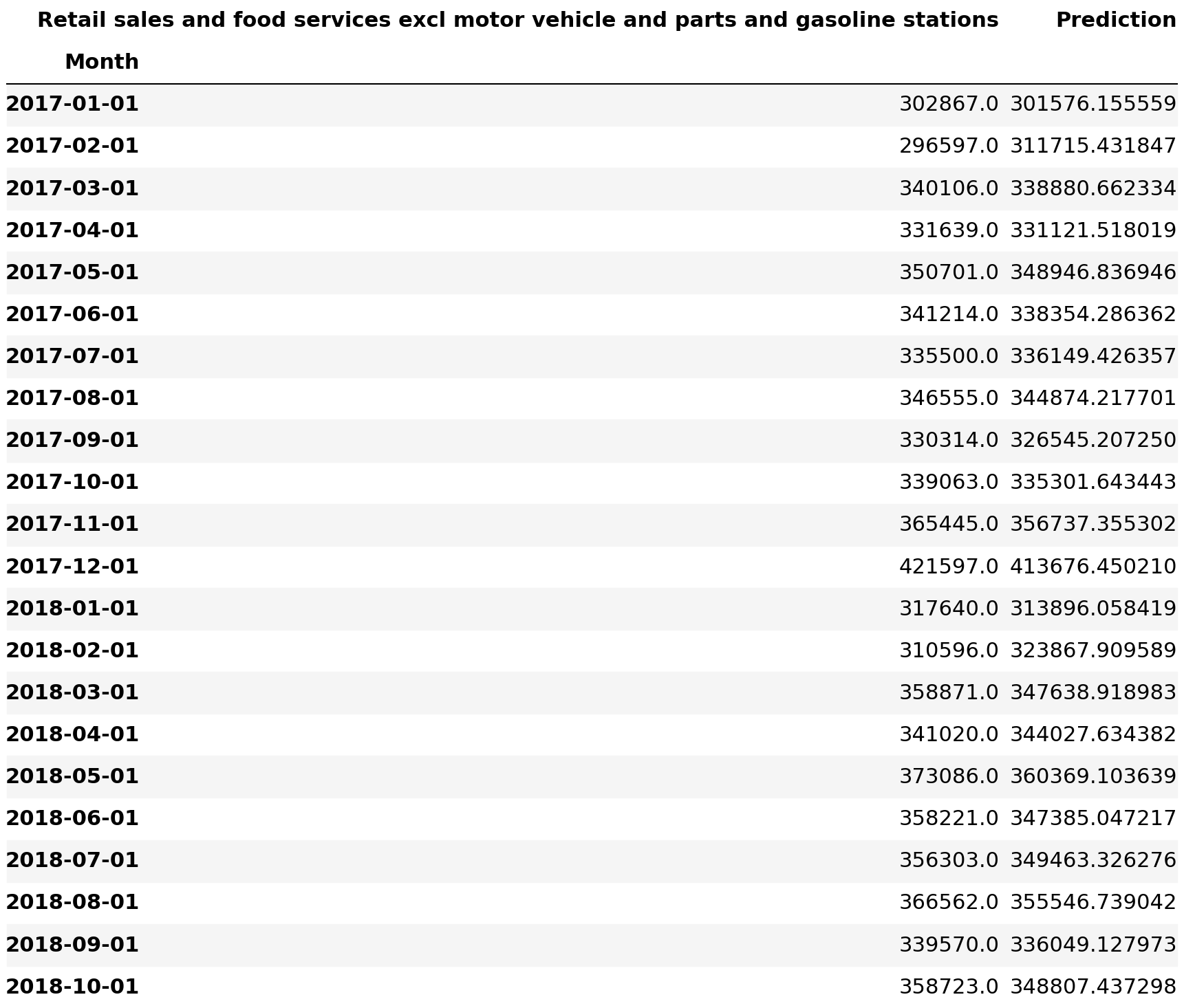

3.7.4.7.2. Plot the differences between historical/actual sales data with forecast

Retail_sales_and_food_services_excl_motor_vehicle_and_parts_and_gasoline_stations_validate.plot()
plt.pyplot.show()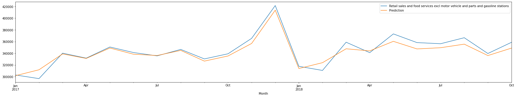

3.7.4.7.3. Compute the absolute difference between actual sales with forecasted sales

Retail_sales_and_food_services_excl_motor_vehicle_and_parts_and_gasoline_stations_validate['Abs Diff'] = (Retail_sales_and_food_services_excl_motor_vehicle_and_parts_and_gasoline_stations_validate['Retail sales and food services excl motor vehicle and parts and gasoline stations'] - Retail_sales_and_food_services_excl_motor_vehicle_and_parts_and_gasoline_stations_validate['Prediction']).abs()
Retail_sales_and_food_services_excl_motor_vehicle_and_parts_and_gasoline_stations_validate['Abs Diff %'] = (Retail_sales_and_food_services_excl_motor_vehicle_and_parts_and_gasoline_stations_validate['Retail sales and food services excl motor vehicle and parts and gasoline stations'] - Retail_sales_and_food_services_excl_motor_vehicle_and_parts_and_gasoline_stations_validate['Prediction']).abs()/Retail_sales_and_food_services_excl_motor_vehicle_and_parts_and_gasoline_stations_validate['Retail sales and food services excl motor vehicle and parts and gasoline stations']
Retail_sales_and_food_services_excl_motor_vehicle_and_parts_and_gasoline_stations_validate.loc['Average Abs Diff %'] = pd.Series(Retail_sales_and_food_services_excl_motor_vehicle_and_parts_and_gasoline_stations_validate['Abs Diff %'].mean(), index = ['Abs Diff %'])
Retail_sales_and_food_services_excl_motor_vehicle_and_parts_and_gasoline_stations_validate.loc['Min Abs Diff %'] = pd.Series(Retail_sales_and_food_services_excl_motor_vehicle_and_parts_and_gasoline_stations_validate['Abs Diff %'].min(), index = ['Abs Diff %'])
Retail_sales_and_food_services_excl_motor_vehicle_and_parts_and_gasoline_stations_validate.loc['Max Abs Diff %'] = pd.Series(Retail_sales_and_food_services_excl_motor_vehicle_and_parts_and_gasoline_stations_validate['Abs Diff %'].max(), index = ['Abs Diff %'])
Retail_sales_and_food_services_excl_motor_vehicle_and_parts_and_gasoline_stations_validate

3.7.4.7.4. Compare all historical/actual sales data with forecast

Retail_sales_and_food_services_excl_motor_vehicle_and_parts_and_gasoline_stations = monthly_retail_data.filter(items=['Retail sales and food services excl motor vehicle and parts and gasoline stations'])
Retail_sales_and_food_services_excl_motor_vehicle_and_parts_and_gasoline_stations_1 = Retail_sales_and_food_services_excl_motor_vehicle_and_parts_and_gasoline_stations.loc['2005-01-01':'2016-12-01']
Retail_sales_and_food_services_excl_motor_vehicle_and_parts_and_gasoline_stations_2 = Retail_sales_and_food_services_excl_motor_vehicle_and_parts_and_gasoline_stations.loc['2017-01-01':]Retail_sales_and_food_services_excl_motor_vehicle_and_parts_and_gasoline_stations_forecast_all = Retail_sales_and_food_services_excl_motor_vehicle_and_parts_and_gasoline_stations_fit.predict(n_periods=48)
Retail_sales_and_food_services_excl_motor_vehicle_and_parts_and_gasoline_stations_forecast_allarray([301576.1555587 , 311715.43184672, 338880.66233398, 331121.51801881,
       348946.83694635, 338354.28636231, 336149.42635728, 344874.21770071,
       326545.2072504 , 335301.64344331, 356737.35530158, 413676.4502102 ,
       313896.05841907, 323867.90958886, 347638.91898302, 344027.63438206,
       360369.10363905, 347385.04721719, 349463.32627588, 355546.73904208,
       336049.12797276, 348807.43729806, 366713.46384   , 423806.03665247,
       327361.74476763, 333267.8000903 , 358484.30424787, 357227.76357623,
       369367.4192089 , 358965.97540448, 362200.76886428, 364355.02441998,
       348313.84998651, 360932.15837247, 375559.24493626, 436637.14562984,
       338784.79962074, 342372.35550155, 371710.86547933, 367929.21354882,
       378924.41244763, 372380.70315779, 372230.82027971, 374512.05727888,
       361693.60899075, 370405.49207768, 386404.08570605, 449764.75264076])Retail_sales_and_food_services_excl_motor_vehicle_and_parts_and_gasoline_stations_validate_all = pd.DataFrame(Retail_sales_and_food_services_excl_motor_vehicle_and_parts_and_gasoline_stations_forecast_all, index = Retail_sales_and_food_services_excl_motor_vehicle_and_parts_and_gasoline_stations_2.index, columns=['Prediction'])
Retail_sales_and_food_services_excl_motor_vehicle_and_parts_and_gasoline_stations_validate_all = pd.concat([Retail_sales_and_food_services_excl_motor_vehicle_and_parts_and_gasoline_stations_2, Retail_sales_and_food_services_excl_motor_vehicle_and_parts_and_gasoline_stations_validate_all], axis=1)
Retail_sales_and_food_services_excl_motor_vehicle_and_parts_and_gasoline_stations_validate_all = Retail_sales_and_food_services_excl_motor_vehicle_and_parts_and_gasoline_stations_1.append(Retail_sales_and_food_services_excl_motor_vehicle_and_parts_and_gasoline_stations_validate_all, sort=True)Retail_sales_and_food_services_excl_motor_vehicle_and_parts_and_gasoline_stations_validate_all.plot()
plt.pyplot.show()

3.7.5. Retail sales, total

3.7.5.1. Filter Monthly Retail Data to just Retail sales, total data

Retail_sales_total_data = monthly_retail_actuals.filter(items=['Retail sales, total'])print('All: ', Retail_sales_total_data.shape)All:  (166, 1)

3.7.5.2. Split the data into Train and Test data

We will be diving data into two sets of data:

Train Data
Train Data
Test Data
Test Data

Train Data: January 2005 thru December 2016
Train Data: January 2005 thru December 2016
Test Data: January 2017 thru October 2018
Test Data: January 2017 thru October 2018

Retail_sales_total_train = Retail_sales_total_data.loc['2005-01-01':'2016-12-01']
Retail_sales_total_test = Retail_sales_total_data.loc['2017-01-01':]

3.7.5.3. Validate data split was done correctly

print( 'Train: ', Retail_sales_total_train.shape)
print( 'Test: ', Retail_sales_total_test.shape)Train:  (144, 1)
Test:  (22, 1)

3.7.5.4. Train Forecast Model for Retail and food services sales, total using ARIMA (Autoregressive Integrated Moving Average) Model to find optimal Hyper-Parameters

ARIMA Model is bit difficult to explain, but it is best way to create a forecast of times series data. If you want to know more, here goes:

AR: Autoregression. A model that uses the dependent relationship between an observation and some number of lagged observations.
AR: Autoregression. A model that uses the dependent relationship between an observation and some number of lagged observations.
I: Integrated. The use of differencing of raw observations (e.g. subtracting an observation from an observation at the previous time step) in order to make the time series stationary.
I: Integrated. The use of differencing of raw observations (eg subtracting an observation from an observation at the previous time step) in order to make the time series stationary.
MA: Moving Average. A model that uses the dependency between an observation and a residual error from a moving average model applied to lagged observations.
MA: Moving Average. A model that uses the dependency between an observation and a residual error from a moving average model applied to lagged observations.

3.7.5.4.1. Find the best fit using brute force search using train data

Please note the parameters used:

m=12 (Denote that retail sales data is monthly)
m=12 (Denote that retail sales data is monthly)
seasonal=True (Denotes that retail sales data has seasonality)
seasonal=True (Denotes that retail sales data has seasonality)
d=1 (Denotes that retail sales data is not stationary and differencing of 1 is required as noted on section 3.5.11.3)
d=1 (Denotes that retail sales data is not stationary and differencing of 1 is required as noted on section 3.5.11.3)
stepwise=False (Denotes brute force search since dataset is small, not intelligent search)
stepwise=False (Denotes brute force search since dataset is small, not intelligent search)

Retail_sales_total_fit = pm.auto_arima(Retail_sales_total_train,
                           m=12,
                           seasonal=True,
                           d=1, 
                           trace=True,
                           error_action='ignore',  
                           suppress_warnings=True, 
                           stepwise=False)ARIMA(0,1,0)(0,1,0)[12]             : AIC=2746.175, Time=0.11 sec
 ARIMA(0,1,0)(0,1,1)[12]             : AIC=2749.897, Time=0.46 sec
 ARIMA(0,1,0)(0,1,2)[12]             : AIC=2747.325, Time=1.48 sec
 ARIMA(0,1,0)(1,1,0)[12]             : AIC=2747.885, Time=0.29 sec
 ARIMA(0,1,0)(1,1,1)[12]             : AIC=2747.595, Time=2.39 sec
 ARIMA(0,1,0)(1,1,2)[12]             : AIC=2746.642, Time=2.24 sec
 ARIMA(0,1,0)(2,1,0)[12]             : AIC=2747.562, Time=0.55 sec
 ARIMA(0,1,0)(2,1,1)[12]             : AIC=2752.613, Time=2.35 sec
 ARIMA(0,1,0)(2,1,2)[12]             : AIC=2746.041, Time=3.95 sec
 ARIMA(0,1,1)(0,1,0)[12]             : AIC=2748.280, Time=0.07 sec
 ARIMA(0,1,1)(0,1,1)[12]             : AIC=2750.268, Time=0.40 sec
 ARIMA(0,1,1)(0,1,2)[12]             : AIC=2749.511, Time=0.98 sec
 ARIMA(0,1,1)(1,1,0)[12]             : AIC=2750.269, Time=0.26 sec
 ARIMA(0,1,1)(1,1,1)[12]             : AIC=2749.793, Time=0.78 sec
 ARIMA(0,1,1)(1,1,2)[12]             : AIC=2748.636, Time=1.89 sec
 ARIMA(0,1,1)(2,1,0)[12]             : AIC=2749.794, Time=0.86 sec
 ARIMA(0,1,1)(2,1,1)[12]             : AIC=2748.195, Time=1.87 sec
 ARIMA(0,1,1)(2,1,2)[12]             : AIC=2747.105, Time=5.26 sec
 ARIMA(0,1,2)(0,1,0)[12]             : AIC=2749.774, Time=0.26 sec
 ARIMA(0,1,2)(0,1,1)[12]             : AIC=2751.740, Time=0.50 sec
 ARIMA(0,1,2)(0,1,2)[12]             : AIC=2750.983, Time=2.09 sec
 ARIMA(0,1,2)(1,1,0)[12]             : AIC=2751.743, Time=0.35 sec
 ARIMA(0,1,2)(1,1,1)[12]             : AIC=2751.058, Time=0.90 sec
 ARIMA(0,1,2)(1,1,2)[12]             : AIC=2750.115, Time=1.99 sec
 ARIMA(0,1,2)(2,1,0)[12]             : AIC=2751.302, Time=0.94 sec
 ARIMA(0,1,2)(2,1,1)[12]             : AIC=2749.704, Time=1.94 sec
 ARIMA(0,1,3)(0,1,0)[12]             : AIC=2749.158, Time=0.15 sec
 ARIMA(0,1,3)(0,1,1)[12]             : AIC=2751.091, Time=0.63 sec
 ARIMA(0,1,3)(0,1,2)[12]             : AIC=2750.646, Time=1.40 sec
 ARIMA(0,1,3)(1,1,0)[12]             : AIC=2751.096, Time=0.39 sec
 ARIMA(0,1,3)(1,1,1)[12]             : AIC=2750.497, Time=1.44 sec
 ARIMA(0,1,3)(2,1,0)[12]             : AIC=2750.949, Time=1.28 sec
 ARIMA(0,1,4)(0,1,0)[12]             : AIC=2747.838, Time=0.22 sec
 ARIMA(0,1,4)(0,1,1)[12]             : AIC=2749.736, Time=0.81 sec
 ARIMA(0,1,4)(1,1,0)[12]             : AIC=2749.743, Time=0.48 sec
 ARIMA(0,1,5)(0,1,0)[12]             : AIC=2747.473, Time=0.25 sec
 ARIMA(1,1,0)(0,1,0)[12]             : AIC=2748.695, Time=0.10 sec
 ARIMA(1,1,0)(0,1,1)[12]             : AIC=2750.684, Time=0.36 sec
 ARIMA(1,1,0)(0,1,2)[12]             : AIC=2749.854, Time=0.87 sec
 ARIMA(1,1,0)(1,1,0)[12]             : AIC=2750.684, Time=0.29 sec
 ARIMA(1,1,0)(1,1,1)[12]             : AIC=2750.148, Time=0.66 sec
 ARIMA(1,1,0)(1,1,2)[12]             : AIC=2748.904, Time=1.82 sec
 ARIMA(1,1,0)(2,1,0)[12]             : AIC=2750.144, Time=0.83 sec
 ARIMA(1,1,0)(2,1,1)[12]             : AIC=2748.451, Time=1.78 sec
 ARIMA(1,1,0)(2,1,2)[12]             : AIC=2747.266, Time=4.19 sec
 ARIMA(1,1,1)(0,1,0)[12]             : AIC=2750.476, Time=0.26 sec
 ARIMA(1,1,1)(0,1,1)[12]             : AIC=2752.461, Time=1.55 sec
 ARIMA(1,1,1)(0,1,2)[12]             : AIC=2751.645, Time=2.29 sec
 ARIMA(1,1,1)(1,1,0)[12]             : AIC=2752.462, Time=0.88 sec
 ARIMA(1,1,1)(1,1,1)[12]             : AIC=2751.891, Time=2.44 sec
 ARIMA(1,1,1)(1,1,2)[12]             : AIC=2750.713, Time=3.63 sec
 ARIMA(1,1,1)(2,1,0)[12]             : AIC=2751.941, Time=2.95 sec
 ARIMA(1,1,1)(2,1,1)[12]             : AIC=2750.269, Time=3.46 sec
 ARIMA(1,1,2)(0,1,0)[12]             : AIC=2748.672, Time=0.30 sec
 ARIMA(1,1,2)(0,1,1)[12]             : AIC=2750.596, Time=1.21 sec
 ARIMA(1,1,2)(0,1,2)[12]             : AIC=2749.922, Time=2.61 sec
 ARIMA(1,1,2)(1,1,0)[12]             : AIC=2750.602, Time=1.48 sec
 ARIMA(1,1,2)(1,1,1)[12]             : AIC=2749.780, Time=2.47 sec
 ARIMA(1,1,2)(2,1,0)[12]             : AIC=2750.256, Time=3.44 sec
 ARIMA(1,1,3)(0,1,0)[12]             : AIC=2749.117, Time=0.61 sec
 ARIMA(1,1,3)(0,1,1)[12]             : AIC=2751.035, Time=2.30 sec
 ARIMA(1,1,3)(1,1,0)[12]             : AIC=2751.041, Time=0.89 sec
 ARIMA(1,1,4)(0,1,0)[12]             : AIC=2749.165, Time=0.81 sec
 ARIMA(2,1,0)(0,1,0)[12]             : AIC=2750.759, Time=0.10 sec
 ARIMA(2,1,0)(0,1,1)[12]             : AIC=2752.722, Time=0.85 sec
 ARIMA(2,1,0)(0,1,2)[12]             : AIC=2751.788, Time=1.13 sec
 ARIMA(2,1,0)(1,1,0)[12]             : AIC=2752.725, Time=0.38 sec
 ARIMA(2,1,0)(1,1,1)[12]             : AIC=2751.871, Time=1.13 sec
 ARIMA(2,1,0)(1,1,2)[12]             : AIC=2750.737, Time=2.06 sec
 ARIMA(2,1,0)(2,1,0)[12]             : AIC=2752.128, Time=1.13 sec
 ARIMA(2,1,0)(2,1,1)[12]             : AIC=2750.299, Time=4.13 sec
 ARIMA(2,1,1)(0,1,0)[12]             : AIC=2751.701, Time=0.35 sec
 ARIMA(2,1,1)(0,1,1)[12]             : AIC=2753.589, Time=1.24 sec
 ARIMA(2,1,1)(0,1,2)[12]             : AIC=2752.506, Time=3.19 sec
 ARIMA(2,1,1)(1,1,0)[12]             : AIC=2753.598, Time=1.31 sec
 ARIMA(2,1,1)(1,1,1)[12]             : AIC=2752.283, Time=1.87 sec
 ARIMA(2,1,1)(2,1,0)[12]             : AIC=2752.906, Time=4.65 sec
 ARIMA(2,1,2)(0,1,0)[12]             : AIC=2700.034, Time=1.00 sec
 ARIMA(2,1,2)(0,1,1)[12]             : AIC=2702.572, Time=2.49 sec
 ARIMA(2,1,2)(1,1,0)[12]             : AIC=2701.823, Time=3.17 sec
 ARIMA(2,1,3)(0,1,0)[12]             : AIC=2701.728, Time=1.31 sec
 ARIMA(3,1,0)(0,1,0)[12]             : AIC=2752.371, Time=0.14 sec
 ARIMA(3,1,0)(0,1,1)[12]             : AIC=2754.298, Time=0.46 sec
 ARIMA(3,1,0)(0,1,2)[12]             : AIC=2753.440, Time=1.32 sec
 ARIMA(3,1,0)(1,1,0)[12]             : AIC=2754.303, Time=0.49 sec
 ARIMA(3,1,0)(1,1,1)[12]             : AIC=2753.300, Time=1.24 sec
 ARIMA(3,1,0)(2,1,0)[12]             : AIC=2753.790, Time=1.39 sec
 ARIMA(3,1,1)(0,1,0)[12]             : AIC=2751.000, Time=0.41 sec
 ARIMA(3,1,1)(0,1,1)[12]             : AIC=2752.882, Time=1.98 sec
 ARIMA(3,1,1)(1,1,0)[12]             : AIC=2752.891, Time=1.23 sec
 ARIMA(3,1,2)(0,1,0)[12]             : AIC=2700.106, Time=1.20 sec
 ARIMA(4,1,0)(0,1,0)[12]             : AIC=2750.147, Time=0.25 sec
 ARIMA(4,1,0)(0,1,1)[12]             : AIC=2751.997, Time=0.68 sec
 ARIMA(4,1,0)(1,1,0)[12]             : AIC=2752.007, Time=0.77 sec
 ARIMA(4,1,1)(0,1,0)[12]             : AIC=2751.075, Time=0.54 sec
 ARIMA(5,1,0)(0,1,0)[12]             : AIC=2749.003, Time=0.30 sec
Total fit time: 130.782 seconds

3.7.5.4.2. View the summary of selected optimal hyper-parameters

Retail_sales_total_fit.summary()

SARIMAX Results Dep. Variable: y No. Observations: 144 Model: SARIMAX(2, 1, 2)x(0, 1, [], 12) Log Likelihood -1345.017 Date: Sat, 15 Aug 2020 AIC 2700.034 Time: 15:17:07 BIC 2714.410 Sample: 0 HQIC 2705.876–144 Covariance Type: opg coef std err z P>|z| [0.025 0.975] ar.L1 -1.1704 0.010 -117.542 0.000 -1.190 -1.151 ar.L2 -0.9927 0.009 -110.808 0.000 -1.010 -0.975 ma.L1 1.1585 0.056 20.524 0.000 1.048 1.269 ma.L2 0.9977 0.100 9.962 0.000 0.801 1.194 sigma2 5.853e+07 1.13e-09 5.19e+16 0.000 5.85e+07 5.85e+07 Ljung-Box (Q): 43.23 Jarque-Bera (JB): 2.97 Prob(Q): 0.33 Prob(JB): 0.23 Heteroskedasticity (H): 0.70 Skew: -0.15 Prob(H) (two-sided): 0.24 Kurtosis: 3.67 Warnings:[1] Covariance matrix calculated using the outer product of gradients (complex-step).[2] Covariance matrix is singular or near-singular, with condition number 3.56e+32. Standard errors may be unstable.

3.7.5.5. Fit Forecast Model

Retail_sales_total_fit.fit(Retail_sales_total_train)ARIMA(maxiter=50, method='lbfgs', order=(2, 1, 2), out_of_sample_size=0,
      scoring='mse', scoring_args={}, seasonal_order=(0, 1, 0, 12),
      start_params=None, suppress_warnings=True, trend=None,
      with_intercept=False)

3.7.5.6. Predict Forecast

Retail_sales_total_forecast = Retail_sales_total_fit.predict(n_periods=22)Retail_sales_total_forecastarray([370554.60086878, 387088.61064245, 423365.76283075, 414783.91551886,
       436622.62786759, 427772.42211495, 426966.33120343, 439538.204078  ,
       411773.46009053, 419357.16442082, 436703.5656634 , 500975.84384621,
       392785.37020954, 407753.44881669, 440606.20409843, 437586.88383178,
       456314.37928796, 445583.7829162 , 450067.04923991, 458314.71124638,
       430360.48287816, 442458.57430173])

3.7.5.7. Validate Forecast

3.7.5.7.1. Compare historical/actual sales data with forecast

Retail_sales_total_validate = pd.DataFrame(Retail_sales_total_forecast, index = Retail_sales_total_test.index, columns=['Prediction'])
Retail_sales_total_validate = pd.concat([Retail_sales_total_test, Retail_sales_total_validate], axis=1)
Retail_sales_total_validate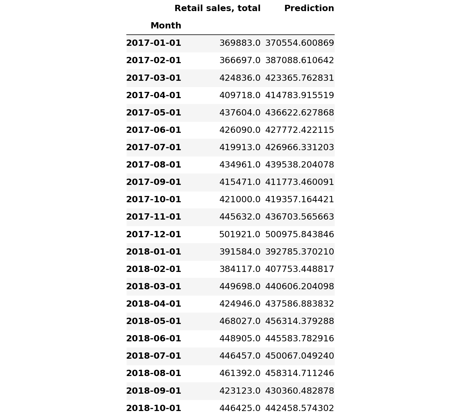

3.7.5.7.2. Plot the differences between historical/actual sales data with forecast

Retail_sales_total_validate.plot()
plt.pyplot.show()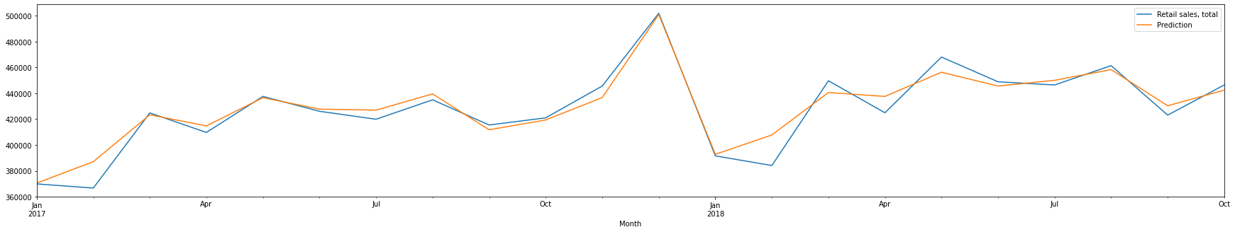

3.7.5.7.3. Compute the absolute difference between actual sales with forecasted sales

Retail_sales_total_validate['Abs Diff'] = (Retail_sales_total_validate['Retail sales, total'] - Retail_sales_total_validate['Prediction']).abs()
Retail_sales_total_validate['Abs Diff %'] = (Retail_sales_total_validate['Retail sales, total'] - Retail_sales_total_validate['Prediction']).abs()/Retail_sales_total_validate['Retail sales, total']
Retail_sales_total_validate.loc['Average Abs Diff %'] = pd.Series(Retail_sales_total_validate['Abs Diff %'].mean(), index = ['Abs Diff %'])
Retail_sales_total_validate.loc['Min Abs Diff %'] = pd.Series(Retail_sales_total_validate['Abs Diff %'].min(), index = ['Abs Diff %'])
Retail_sales_total_validate.loc['Max Abs Diff %'] = pd.Series(Retail_sales_total_validate['Abs Diff %'].max(), index = ['Abs Diff %'])
Retail_sales_total_validate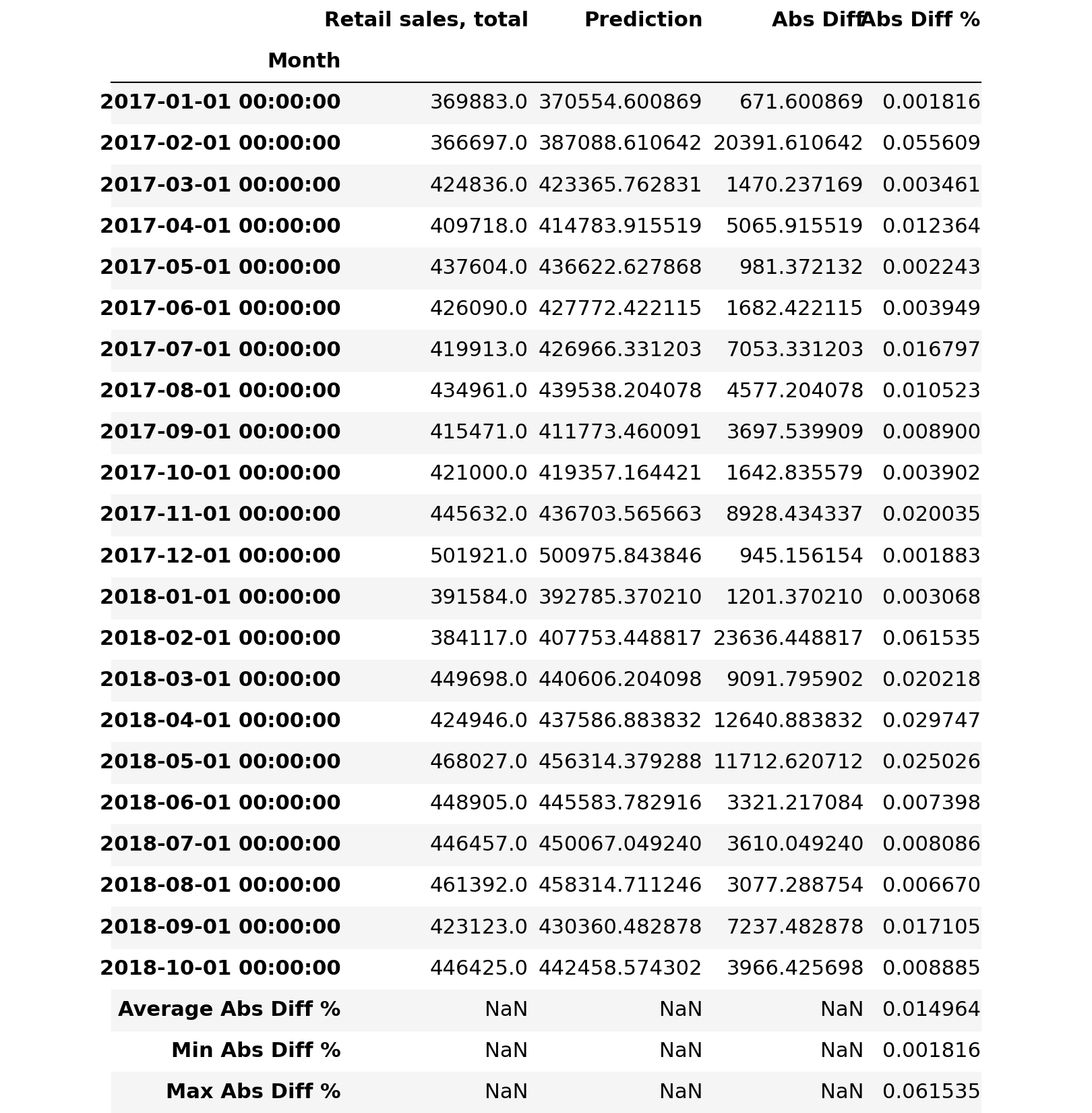

3.7.5.7.4. Compare all historical/actual sales data with forecast.

Retail_sales_total = monthly_retail_data.filter(items=['Retail sales, total'])
Retail_sales_total_1 = Retail_sales_total.loc['2005-01-01':'2016-12-01']
Retail_sales_total_2 = Retail_sales_total.loc['2017-01-01':]Retail_sales_total_forecast_all = Retail_sales_total_fit.predict(n_periods=48)
Retail_sales_total_forecast_allarray([370554.60086878, 387088.61064245, 423365.76283075, 414783.91551886,
       436622.62786759, 427772.42211495, 426966.33120343, 439538.204078  ,
       411773.46009053, 419357.16442082, 436703.5656634 , 500975.84384621,
       392785.37020954, 407753.44881669, 440606.20409843, 437586.88383178,
       456314.37928796, 445583.7829162 , 450067.04923991, 458314.71124638,
       430360.48287816, 442458.57430173, 454709.2699724 , 520464.35593458,
       415596.8132566 , 425203.6401893 , 461032.75663688, 459851.86274478,
       473472.98760526, 466894.0853423 , 471587.10673242, 475467.91201677,
       452416.59169573, 463111.08051925, 472137.52904234, 543059.73719544,
       435345.08707203, 443154.91500758, 483913.60484479, 478746.82220555,
       492139.63238294, 489784.71612043, 489760.47459881, 494969.42312937,
       475046.38200893, 480760.98092825, 492510.65989448, 565188.99334718])Retail_sales_total_validate_all = pd.DataFrame(Retail_sales_total_forecast_all, index = Retail_sales_total_2.index, columns=['Prediction'])
Retail_sales_total_validate_all = pd.concat([Retail_sales_total_2, Retail_sales_total_validate_all], axis=1)
Retail_sales_total_validate_all = Retail_sales_total_1.append(Retail_sales_total_validate_all, sort=True)Retail_sales_total_validate_all.plot()
plt.pyplot.show()

3.7.6. Retail sales, total (excl. motor vehicle and parts dealers)

3.7.6.1. Filter Monthly Retail Data to just Retail sales, total (excl. motor vehicle and parts dealers) data

Retail_sales_total_excl_motor_vehicle_and_parts_dealers_data = monthly_retail_actuals.filter(items=['Retail sales, total (excl. motor vehicle and parts dealers)'])print('All: ', Retail_sales_total_excl_motor_vehicle_and_parts_dealers_data.shape)All:  (166, 1)

3.7.6.2. Split the data into Train and Test data

We will be diving data into two sets of data:

Train Data
Train Data
Test Data
Test Data

Train Data: January 2005 thru December 2016
Train Data: January 2005 thru December 2016
Test Data: January 2017 thru October 2018
Test Data: January 2017 thru October 2018

Retail_sales_total_excl_motor_vehicle_and_parts_dealers_train = Retail_sales_total_excl_motor_vehicle_and_parts_dealers_data.loc['2005-01-01':'2016-12-01']
Retail_sales_total_excl_motor_vehicle_and_parts_dealers_test = Retail_sales_total_excl_motor_vehicle_and_parts_dealers_data.loc['2017-01-01':]

3.7.6.3. Validate data split was done correctly

print( 'Train: ', Retail_sales_total_excl_motor_vehicle_and_parts_dealers_train.shape)
print( 'Test: ', Retail_sales_total_excl_motor_vehicle_and_parts_dealers_test.shape)Train:  (144, 1)
Test:  (22, 1)

3.7.6.4. Train Forecast Model for Retail and food services sales, total using ARIMA (Autoregressive Integrated Moving Average) Model to find optimal Hyper-Parameters

ARIMA Model is bit difficult to explain, but it is best way to create a forecast of times series data. If you want to know more, here goes:

AR: Autoregression. A model that uses the dependent relationship between an observation and some number of lagged observations.
AR: Autoregression. A model that uses the dependent relationship between an observation and some number of lagged observations.
I: Integrated. The use of differencing of raw observations (e.g. subtracting an observation from an observation at the previous time step) in order to make the time series stationary.
I: Integrated. The use of differencing of raw observations (eg subtracting an observation from an observation at the previous time step) in order to make the time series stationary.
MA: Moving Average. A model that uses the dependency between an observation and a residual error from a moving average model applied to lagged observations.
MA: Moving Average. A model that uses the dependency between an observation and a residual error from a moving average model applied to lagged observations.

3.7.6.4.1. Find the best fit using brute force search using train data

Please note the parameters used:

m=12 (Denote that retail sales data is monthly)
m=12 (Denote that retail sales data is monthly)
seasonal=True (Denotes that retail sales data has seasonality)
seasonal=True (Denotes that retail sales data has seasonality)
stepwise=False (Denotes brute force search since dataset is small, not intelligent search)
stepwise=False (Denotes brute force search since dataset is small, not intelligent search)
d = 1 (Denotes that data is not stationary and differencing of data is needed, despite ADF test. KPSS test recommends d=’1')
d = 1 (Denotes that data is not stationary and differencing of data is needed, despite ADF test. KPSS test recommends d='1')

Retail_sales_total_excl_motor_vehicle_and_parts_dealers_fit = pm.auto_arima(Retail_sales_total_excl_motor_vehicle_and_parts_dealers_train, 
                           m=12,
                           seasonal=True,
                           d=1,
                           trace=True,
                           error_action='ignore',  
                           suppress_warnings=True, 
                           stepwise=False)ARIMA(0,1,0)(0,1,0)[12]             : AIC=2659.319, Time=0.06 sec
 ARIMA(0,1,0)(0,1,1)[12]             : AIC=2664.471, Time=0.27 sec
 ARIMA(0,1,0)(0,1,2)[12]             : AIC=2661.313, Time=0.67 sec
 ARIMA(0,1,0)(1,1,0)[12]             : AIC=2661.452, Time=0.13 sec
 ARIMA(0,1,0)(1,1,1)[12]             : AIC=2667.339, Time=0.47 sec
 ARIMA(0,1,0)(1,1,2)[12]             : AIC=2660.870, Time=1.45 sec
 ARIMA(0,1,0)(2,1,0)[12]             : AIC=2661.187, Time=0.55 sec
 ARIMA(0,1,0)(2,1,1)[12]             : AIC=2668.999, Time=1.17 sec
 ARIMA(0,1,0)(2,1,2)[12]             : AIC=2659.127, Time=4.62 sec
 ARIMA(0,1,1)(0,1,0)[12]             : AIC=2661.263, Time=0.07 sec
 ARIMA(0,1,1)(0,1,1)[12]             : AIC=2663.263, Time=0.36 sec
 ARIMA(0,1,1)(0,1,2)[12]             : AIC=2662.926, Time=1.01 sec
 ARIMA(0,1,1)(1,1,0)[12]             : AIC=2663.263, Time=0.23 sec
 ARIMA(0,1,1)(1,1,1)[12]             : AIC=2663.506, Time=0.65 sec
 ARIMA(0,1,1)(1,1,2)[12]             : AIC=2662.467, Time=1.81 sec
 ARIMA(0,1,1)(2,1,0)[12]             : AIC=2663.070, Time=0.74 sec
 ARIMA(0,1,1)(2,1,1)[12]             : AIC=2662.074, Time=2.34 sec
 ARIMA(0,1,1)(2,1,2)[12]             : AIC=2659.491, Time=5.53 sec
 ARIMA(0,1,2)(0,1,0)[12]             : AIC=2662.964, Time=0.19 sec
 ARIMA(0,1,2)(0,1,1)[12]             : AIC=2664.962, Time=0.92 sec
 ARIMA(0,1,2)(0,1,2)[12]             : AIC=2664.630, Time=1.19 sec
 ARIMA(0,1,2)(1,1,0)[12]             : AIC=2664.962, Time=0.32 sec
 ARIMA(0,1,2)(1,1,1)[12]             : AIC=2665.061, Time=0.90 sec
 ARIMA(0,1,2)(1,1,2)[12]             : AIC=2664.216, Time=2.17 sec
 ARIMA(0,1,2)(2,1,0)[12]             : AIC=2664.799, Time=0.89 sec
 ARIMA(0,1,2)(2,1,1)[12]             : AIC=2663.848, Time=2.97 sec
 ARIMA(0,1,3)(0,1,0)[12]             : AIC=2663.725, Time=0.14 sec
 ARIMA(0,1,3)(0,1,1)[12]             : AIC=2665.717, Time=0.58 sec
 ARIMA(0,1,3)(0,1,2)[12]             : AIC=2665.525, Time=1.44 sec
 ARIMA(0,1,3)(1,1,0)[12]             : AIC=2665.718, Time=0.39 sec
 ARIMA(0,1,3)(1,1,1)[12]             : AIC=2665.815, Time=1.18 sec
 ARIMA(0,1,3)(2,1,0)[12]             : AIC=2665.694, Time=1.21 sec
 ARIMA(0,1,4)(0,1,0)[12]             : AIC=2663.016, Time=0.18 sec
 ARIMA(0,1,4)(0,1,1)[12]             : AIC=2664.997, Time=0.77 sec
 ARIMA(0,1,4)(1,1,0)[12]             : AIC=2664.998, Time=0.44 sec
 ARIMA(0,1,5)(0,1,0)[12]             : AIC=2665.009, Time=0.29 sec
 ARIMA(1,1,0)(0,1,0)[12]             : AIC=2661.436, Time=0.06 sec
 ARIMA(1,1,0)(0,1,1)[12]             : AIC=2663.436, Time=0.33 sec
 ARIMA(1,1,0)(0,1,2)[12]             : AIC=2663.042, Time=0.87 sec
 ARIMA(1,1,0)(1,1,0)[12]             : AIC=2663.436, Time=0.27 sec
 ARIMA(1,1,0)(1,1,1)[12]             : AIC=2663.637, Time=0.60 sec
 ARIMA(1,1,0)(1,1,2)[12]             : AIC=2662.523, Time=1.84 sec
 ARIMA(1,1,0)(2,1,0)[12]             : AIC=2663.188, Time=0.77 sec
 ARIMA(1,1,0)(2,1,1)[12]             : AIC=2662.119, Time=1.66 sec
 ARIMA(1,1,0)(2,1,2)[12]             : AIC=2659.413, Time=4.93 sec
 ARIMA(1,1,1)(0,1,0)[12]             : AIC=2663.287, Time=0.25 sec
 ARIMA(1,1,1)(0,1,1)[12]             : AIC=2665.287, Time=0.84 sec
 ARIMA(1,1,1)(0,1,2)[12]             : AIC=2664.904, Time=2.55 sec
 ARIMA(1,1,1)(1,1,0)[12]             : AIC=2665.286, Time=1.31 sec
 ARIMA(1,1,1)(1,1,1)[12]             : AIC=2665.459, Time=1.38 sec
 ARIMA(1,1,1)(1,1,2)[12]             : AIC=2664.413, Time=4.24 sec
 ARIMA(1,1,1)(2,1,0)[12]             : AIC=2665.057, Time=3.49 sec
 ARIMA(1,1,1)(2,1,1)[12]             : AIC=2664.019, Time=3.54 sec
 ARIMA(1,1,2)(0,1,0)[12]             : AIC=2662.788, Time=0.35 sec
 ARIMA(1,1,2)(0,1,1)[12]             : AIC=2664.739, Time=1.57 sec
 ARIMA(1,1,2)(0,1,2)[12]             : AIC=2664.636, Time=3.32 sec
 ARIMA(1,1,2)(1,1,0)[12]             : AIC=2664.742, Time=1.07 sec
 ARIMA(1,1,2)(1,1,1)[12]             : AIC=2665.105, Time=1.61 sec
 ARIMA(1,1,2)(2,1,0)[12]             : AIC=2664.726, Time=2.98 sec
 ARIMA(1,1,3)(0,1,0)[12]             : AIC=2664.507, Time=0.40 sec
 ARIMA(1,1,3)(0,1,1)[12]             : AIC=2666.494, Time=1.89 sec
 ARIMA(1,1,3)(1,1,0)[12]             : AIC=2666.495, Time=0.95 sec
 ARIMA(1,1,4)(0,1,0)[12]             : AIC=2664.833, Time=0.51 sec
 ARIMA(2,1,0)(0,1,0)[12]             : AIC=2663.302, Time=0.09 sec
 ARIMA(2,1,0)(0,1,1)[12]             : AIC=2665.299, Time=0.41 sec
 ARIMA(2,1,0)(0,1,2)[12]             : AIC=2664.826, Time=1.04 sec
 ARIMA(2,1,0)(1,1,0)[12]             : AIC=2665.300, Time=0.38 sec
 ARIMA(2,1,0)(1,1,1)[12]             : AIC=2665.290, Time=1.03 sec
 ARIMA(2,1,0)(1,1,2)[12]             : AIC=2664.266, Time=2.26 sec
 ARIMA(2,1,0)(2,1,0)[12]             : AIC=2665.005, Time=2.16 sec
 ARIMA(2,1,0)(2,1,1)[12]             : AIC=2663.874, Time=2.64 sec
 ARIMA(2,1,1)(0,1,0)[12]             : AIC=2664.430, Time=0.46 sec
 ARIMA(2,1,1)(0,1,1)[12]             : AIC=2666.374, Time=2.68 sec
 ARIMA(2,1,1)(0,1,2)[12]             : AIC=2665.970, Time=5.08 sec
 ARIMA(2,1,1)(1,1,0)[12]             : AIC=2666.378, Time=1.51 sec
 ARIMA(2,1,1)(1,1,1)[12]             : AIC=2666.421, Time=2.13 sec
 ARIMA(2,1,1)(2,1,0)[12]             : AIC=2666.074, Time=4.00 sec
 ARIMA(2,1,2)(0,1,0)[12]             : AIC=2618.487, Time=0.92 sec
 ARIMA(2,1,2)(0,1,1)[12]             : AIC=2620.347, Time=2.86 sec
 ARIMA(2,1,2)(1,1,0)[12]             : AIC=2621.031, Time=2.66 sec
 ARIMA(2,1,3)(0,1,0)[12]             : AIC=2619.887, Time=1.61 sec
 ARIMA(3,1,0)(0,1,0)[12]             : AIC=2665.374, Time=0.14 sec
 ARIMA(3,1,0)(0,1,1)[12]             : AIC=2667.366, Time=0.53 sec
 ARIMA(3,1,0)(0,1,2)[12]             : AIC=2666.857, Time=1.21 sec
 ARIMA(3,1,0)(1,1,0)[12]             : AIC=2667.367, Time=0.53 sec
 ARIMA(3,1,0)(1,1,1)[12]             : AIC=2667.204, Time=1.23 sec
 ARIMA(3,1,0)(2,1,0)[12]             : AIC=2667.049, Time=1.29 sec
 ARIMA(3,1,1)(0,1,0)[12]             : AIC=2665.455, Time=0.59 sec
 ARIMA(3,1,1)(0,1,1)[12]             : AIC=2667.435, Time=1.33 sec
 ARIMA(3,1,1)(1,1,0)[12]             : AIC=2667.436, Time=1.14 sec
 ARIMA(3,1,2)(0,1,0)[12]             : AIC=2619.664, Time=0.94 sec
 ARIMA(4,1,0)(0,1,0)[12]             : AIC=2664.308, Time=0.23 sec
 ARIMA(4,1,0)(0,1,1)[12]             : AIC=2666.278, Time=0.59 sec
 ARIMA(4,1,0)(1,1,0)[12]             : AIC=2666.280, Time=0.75 sec
 ARIMA(4,1,1)(0,1,0)[12]             : AIC=2665.956, Time=0.58 sec
 ARIMA(5,1,0)(0,1,0)[12]             : AIC=2665.743, Time=0.30 sec
Total fit time: 127.311 seconds

3.7.6.4.2. View the summary of selected optimal hyper-parameters

Retail_sales_total_excl_motor_vehicle_and_parts_dealers_fit.summary()

SARIMAX Results Dep. Variable: y No. Observations: 144 Model: SARIMAX(2, 1, 2)x(0, 1, [], 12) Log Likelihood -1304.243 Date: Sat, 15 Aug 2020 AIC 2618.487 Time: 15:19:16 BIC 2632.862 Sample: 0 HQIC 2624.328–144 Covariance Type: opg coef std err z P>|z| [0.025 0.975] ar.L1 -1.1708 0.011 -110.077 0.000 -1.192 -1.150 ar.L2 -0.9938 0.009 -107.930 0.000 -1.012 -0.976 ma.L1 1.1608 0.051 22.871 0.000 1.061 1.260 ma.L2 0.9980 0.085 11.704 0.000 0.831 1.165 sigma2 3.147e+07 1.82e-09 1.73e+16 0.000 3.15e+07 3.15e+07 Ljung-Box (Q): 60.21 Jarque-Bera (JB): 13.19 Prob(Q): 0.02 Prob(JB): 0.00 Heteroskedasticity (H): 0.64 Skew: -0.34 Prob(H) (two-sided): 0.14 Kurtosis: 4.39 Warnings:[1] Covariance matrix calculated using the outer product of gradients (complex-step).[2] Covariance matrix is singular or near-singular, with condition number 2.13e+31. Standard errors may be unstable.

3.7.6.5. Fit Forecast Model

Retail_sales_total_excl_motor_vehicle_and_parts_dealers_fit.fit(Retail_sales_total_excl_motor_vehicle_and_parts_dealers_train)ARIMA(maxiter=50, method='lbfgs', order=(2, 1, 2), out_of_sample_size=0,
      scoring='mse', scoring_args={}, seasonal_order=(0, 1, 0, 12),
      start_params=None, suppress_warnings=True, trend=None,
      with_intercept=False)

3.7.6.6. Predict Forecast

Retail_sales_total_excl_motor_vehicle_and_parts_dealers_forecast = Retail_sales_total_excl_motor_vehicle_and_parts_dealers_fit.predict(n_periods=22)Retail_sales_total_excl_motor_vehicle_and_parts_dealers_forecastarray([282707.38260801, 288708.26626367, 315715.68838585, 309809.4559079 ,
       329501.95877997, 322664.90660741, 319369.22652367, 327138.5989057 ,
       309391.89947624, 318158.76478208, 338284.8954111 , 393107.50735532,
       296138.59596147, 301242.33972339, 325643.21568741, 323680.38226501,
       341346.27428777, 332963.02728426, 333491.74335077, 338320.04542117,
       320216.08989994, 332324.11384026])

3.7.6.7. Validate Forecast

3.7.6.7.1. Compare historical/actual sales data with forecast

Retail_sales_total_excl_motor_vehicle_and_parts_dealers_validate = pd.DataFrame(Retail_sales_total_excl_motor_vehicle_and_parts_dealers_forecast, index = Retail_sales_total_excl_motor_vehicle_and_parts_dealers_test.index, columns=['Prediction'])
Retail_sales_total_excl_motor_vehicle_and_parts_dealers_validate = pd.concat([Retail_sales_total_excl_motor_vehicle_and_parts_dealers_test, Retail_sales_total_excl_motor_vehicle_and_parts_dealers_validate], axis=1)
Retail_sales_total_excl_motor_vehicle_and_parts_dealers_validate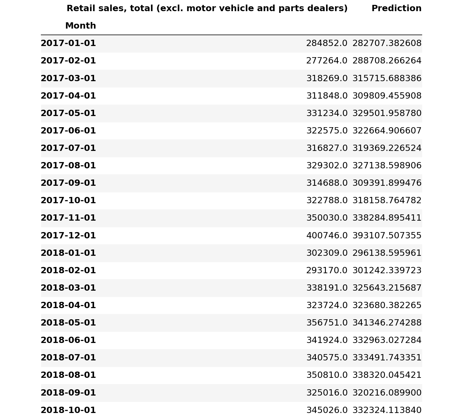

3.7.6.7.2. Plot the differences between historical/actual sales data with forecast

Retail_sales_total_excl_motor_vehicle_and_parts_dealers_validate.plot()
plt.pyplot.show()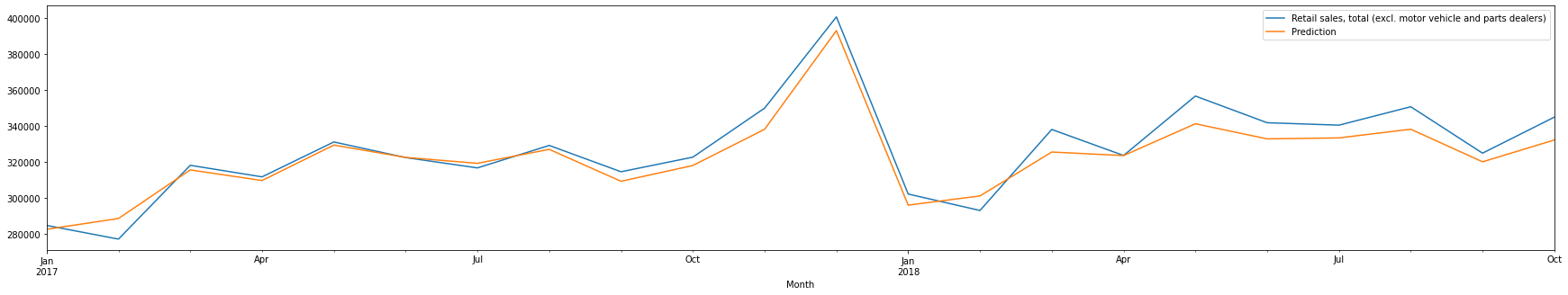

3.7.6.7.3. Compute the absolute difference between actual sales with forecasted sales

Retail_sales_total_excl_motor_vehicle_and_parts_dealers_validate['Abs Diff'] = (Retail_sales_total_excl_motor_vehicle_and_parts_dealers_validate['Retail sales, total (excl. motor vehicle and parts dealers)'] - Retail_sales_total_excl_motor_vehicle_and_parts_dealers_validate['Prediction']).abs()
Retail_sales_total_excl_motor_vehicle_and_parts_dealers_validate['Abs Diff %'] = (Retail_sales_total_excl_motor_vehicle_and_parts_dealers_validate['Retail sales, total (excl. motor vehicle and parts dealers)'] - Retail_sales_total_excl_motor_vehicle_and_parts_dealers_validate['Prediction']).abs()/Retail_sales_total_excl_motor_vehicle_and_parts_dealers_validate['Retail sales, total (excl. motor vehicle and parts dealers)']
Retail_sales_total_excl_motor_vehicle_and_parts_dealers_validate.loc['Average Abs Diff %'] = pd.Series(Retail_sales_total_excl_motor_vehicle_and_parts_dealers_validate['Abs Diff %'].mean(), index = ['Abs Diff %'])
Retail_sales_total_excl_motor_vehicle_and_parts_dealers_validate.loc['Min Abs Diff %'] = pd.Series(Retail_sales_total_excl_motor_vehicle_and_parts_dealers_validate['Abs Diff %'].min(), index = ['Abs Diff %'])
Retail_sales_total_excl_motor_vehicle_and_parts_dealers_validate.loc['Max Abs Diff %'] = pd.Series(Retail_sales_total_excl_motor_vehicle_and_parts_dealers_validate['Abs Diff %'].max(), index = ['Abs Diff %'])
Retail_sales_total_excl_motor_vehicle_and_parts_dealers_validate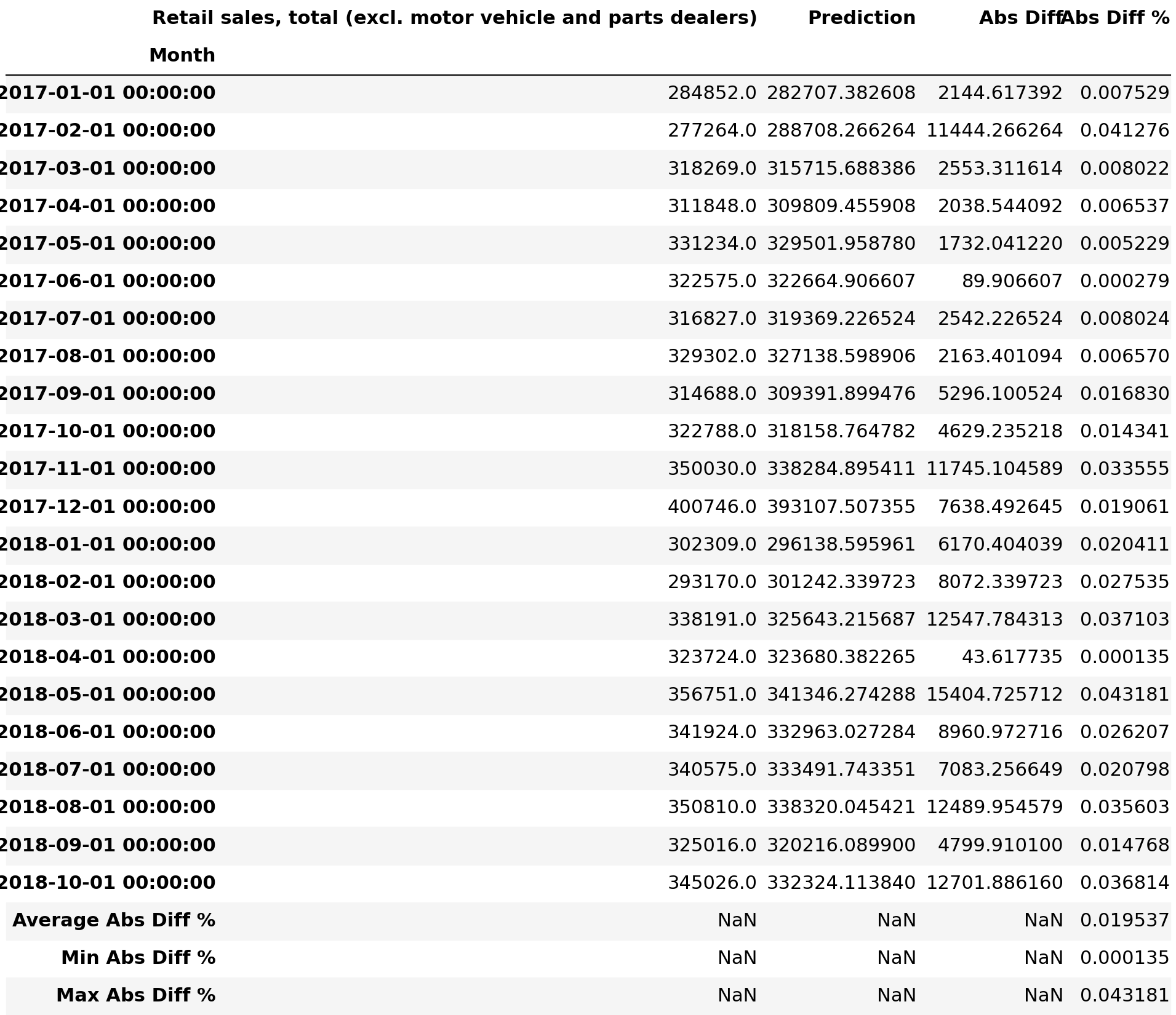

3.7.6.7.4. Compare all historical/actual sales data with forecast

Retail_sales_total_excl_motor_vehicle_and_parts_dealers = monthly_retail_data.filter(items=['Retail sales, total (excl. motor vehicle and parts dealers)'])
Retail_sales_total_excl_motor_vehicle_and_parts_dealers_1 = Retail_sales_total_excl_motor_vehicle_and_parts_dealers.loc['2005-01-01':'2016-12-01']
Retail_sales_total_excl_motor_vehicle_and_parts_dealers_2 = Retail_sales_total_excl_motor_vehicle_and_parts_dealers.loc['2017-01-01':]Retail_sales_total_excl_motor_vehicle_and_parts_dealers_forecast_all = Retail_sales_total_excl_motor_vehicle_and_parts_dealers_fit.predict(n_periods=48)
Retail_sales_total_excl_motor_vehicle_and_parts_dealers_forecast_allarray([282707.38260801, 288708.26626367, 315715.68838585, 309809.4559079 ,
       329501.95877997, 322664.90660741, 319369.22652367, 327138.5989057 ,
       309391.89947624, 318158.76478208, 338284.8954111 , 393107.50735532,
       296138.59596147, 301242.33972339, 325643.21568741, 323680.38226501,
       341346.27428777, 332963.02728426, 333491.74335077, 338320.04542117,
       320216.08989994, 332324.11384026, 348893.37786378, 404559.9712525 ,
       310137.76586457, 311421.00248698, 337764.07428822, 337324.13931442,
       351276.80392189, 345727.62033496, 346628.39790557, 348204.55164834,
       333538.53341828, 344853.36173055, 358934.65195134, 418302.51573165,
       322019.3510503 , 321803.07448292, 351751.25970917, 348580.6033155 ,
       362147.65611619, 359763.78326017, 357341.76164595, 359662.60477398,
       347426.92691362, 355156.16964435, 371020.24934059, 431864.18041473])Retail_sales_total_excl_motor_vehicle_and_parts_dealers_validate_all = pd.DataFrame(Retail_sales_total_excl_motor_vehicle_and_parts_dealers_forecast_all, index = Retail_sales_total_excl_motor_vehicle_and_parts_dealers_2.index, columns=['Prediction'])
Retail_sales_total_excl_motor_vehicle_and_parts_dealers_validate_all = pd.concat([Retail_sales_total_excl_motor_vehicle_and_parts_dealers_2, Retail_sales_total_excl_motor_vehicle_and_parts_dealers_validate_all], axis=1)
Retail_sales_total_excl_motor_vehicle_and_parts_dealers_validate_all = Retail_sales_total_excl_motor_vehicle_and_parts_dealers_1.append(Retail_sales_total_excl_motor_vehicle_and_parts_dealers_validate_all, sort=True)Retail_sales_total_excl_motor_vehicle_and_parts_dealers_validate_all.plot()
plt.pyplot.show()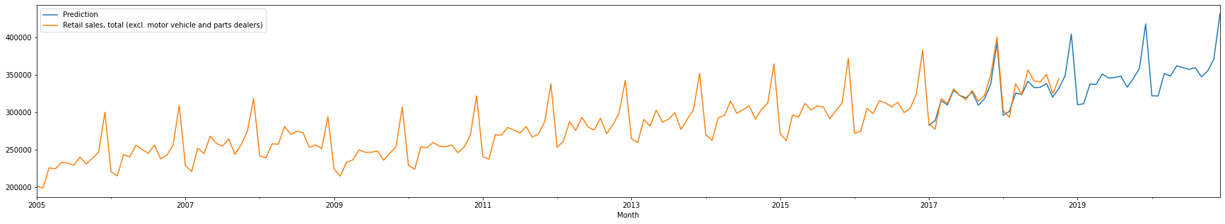

3.8。 Maintain Forecast(3.8. Maintain Forecast)

Like everything, newly created forecast needs to be maintained. More likely on a monthly basis since this is monthly forecast, forecast needs to be updated to reflect revised trend.

To revise the forecast to reflect more up to date data, follow the steps above where you will revise step 3.7.

When diving data into two sets of data:

Train Data: January 2005 thru January 2017 (+ 1 month)
Train Data: January 2005 thru January 2017 (+ 1 month)
Test Data: February 2017 (+ 1 month) thru November 2018 (+ 1 month)
Test Data: February 2017 (+ 1 month) thru November 2018 (+ 1 month)

Repeat the process for all subsequent months.

I hope you have enjoyed this tutorial. If you have any questions or comments, please provide them here.

翻译自: https://medium.com/swlh/create-forecast-using-python-arima-part-2-1-efca5c5c14f3

weixin_26729165

关注

0
点赞
踩
1

收藏

觉得还不错? 一键收藏
0
评论
使用python arima第2部分1创建预测

This tutorial was created to democratize data science for business users (i.e., minimize usage of advanced mathematics topics) and alleviate personal frustration we have experienced on following tutor...
复制链接

扫一扫

使用python arima第2部分1创建预测

1.说明(1. Description)

2.先决条件 (2. Prerequisites)

3.步骤 (3. Steps)

3.1。 获取数据 (3.1. Get Data)

3.2。 格式化数据 (3.2. Format Data)

3.3。 汇入资料 (3.3. Import Data)

3.4。 清理数据 (3.4. Cleanse Data)

3.5。 分析数据(探索性数据分析) (3.5. Analyze Data (Exploratory Data Analysis))

3.6。 准备数据 (3.6. Prep Data)

3.7。 开发和验证预测模型 (3.7. Develop and Validate Forecast Model)

3.8。 Maintain Forecast(3.8. Maintain Forecast)

“相关推荐”对你有帮助么？

3.1。获取数据 (3.1. Get Data)

3.2。格式化数据 (3.2. Format Data)

3.3。汇入资料 (3.3. Import Data)

3.4。清理数据 (3.4. Cleanse Data)

3.5。分析数据(探索性数据分析) (3.5. Analyze Data (Exploratory Data Analysis))

3.6。准备数据 (3.6. Prep Data)

3.7。开发和验证预测模型 (3.7. Develop and Validate Forecast Model)