音乐雷达 shazam算法
Ever wondered how your favorite music searching app works?. Well, this is the correct place to find out.
有没有想过您喜欢的音乐搜索应用程序如何工作? 好吧,这是找出正确的地方。
Ever since I was a kid I was both a music and tech lover. I spent most of my day listening to music and reading about technology. Sometimes I listened to some new song playing around me and I liked it. I wanted to play it but not always Google search was enough to find the song. Then came the Shazam app and it was a great gift to me at the moment. After finding some of my favorite songs playing around, my tech lover side kicked in and wanted to find how it works. After some research, I found out that it uses Machine Learning for music match. After doing more research I got hold of the concepts. Which later motivated me to share the idea with other people as well.
从小我就一直是音乐和科技爱好者。 我大部分时间都在听音乐和阅读有关技术的文章。 有时我听着周围播放的新歌,我很喜欢。 我想播放它,但并非总是Google搜索足以找到歌曲。 然后出现了Shazam应用程序,此刻对我来说是一件很棒的礼物。 在找到我喜欢的一些歌曲后,我的技术爱好者加入了,希望找到它是如何工作的。 经过研究,我发现它使用机器学习进行音乐比赛。 经过更多研究后,我掌握了这些概念。 后来促使我也与其他人分享了这个想法。
So here I am presenting you with brief insights into the concept behind music match apps like Shazam. Here we will build a simple prototype of the music search app using Deep Learning. By the end of the article, you will have complete intuition behind the music search apps.
因此,在这里,我向您简要介绍Shazam等音乐比赛应用背后的概念。 在这里,我们将使用深度学习构建音乐搜索应用程序的简单原型。 到本文结尾,您将全面了解音乐搜索应用程序。
一些基本概念 (Some basic concepts)
短时傅立叶变换(Short Time Fourier Transform)
The Short-time Fourier transform (STFT), is a Fourier-related transform used to determine the sinusoidal frequency and phase content of local sections of a signal as it changes over time. By applying STFT we can decompose a sound wave into its frequencies. The result of this is called a spectrogram. The spectrogram can be thought as a stack of Fast Fourier Transform stack on top of each other. It is a way of visually representing a sound’s loudness or amplitude.
短时傅立叶变换(STFT)是一种与傅立叶相关的变换,用于确定信号随时间变化的局部部分的正弦频率和相位含量。 通过应用STFT,我们可以将声波分解为其频率。 其结果称为频谱图。 频谱图可以看作是彼此快速堆叠的快速傅立叶变换堆栈。 这是一种视觉上代表声音的响度或振幅的方法。
梅尔谱图 (Mel Spectrogram)
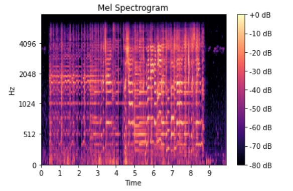
A mel-spectrogram is a spectrogram where the frequencies have been converted into mel-scale. The below image shows a mel-spectrogram of a sound clip.
梅尔频谱图是将频率转换为梅尔标度的频谱图。 下图显示了声音片段的梅尔频谱图。

暹罗神经网络(Siamese Neural Networks)
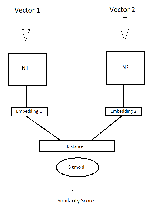
Siamese neural networks are a special kind of network where two identical copies of the same network are fed with different vectors. Instead of recognizing something they learn to find the similarity or difference between two vectors. They are mostly used for one-shot learning.
暹罗神经网络是一种特殊的网络,其中,同一网络的两个相同副本被馈以不同的向量。 他们没有认识到某些东西,而是学会寻找两个向量之间的相似性或差异。 它们主要用于一键式学习。

The neural networks N1 and N2 are essentially having the same architecture. When the input vectors are fed to the network then they both generate feature which is also known as embedding in certain literatures. These neural networks share the same weights and are trained in such a way that that they generate such embeddings that when we calculate the distance for those two embeddings then the distance is minimum for similar vectors and maximum for different vectors.
神经网络N1和N2本质上具有相同的体系结构。 当输入向量被馈送到网络时,它们都将生成特征,这在某些文献中也被称为嵌入。 这些神经网络具有相同的权重,并经过某种方式训练,以使其生成这样的嵌入:当我们为这两个嵌入计算距离时,相似向量的距离最小,而不同向量的距离最大。
总览 (Overview)
Having enough knowledge about the concepts which are going to be used in these article, lets now dive into the details of how this type of system work and how to build our own system.
了解了将在本文中使用的概念的足够知识,现在让我们深入研究此类系统如何工作以及如何构建自己的系统的细节。
Music search engines work on the principle of acoustic fingerprint match in a large database of songs. Whenever we record some sound then the music is processed by an algorithm which converts the music to some sort of acoustic fingerprint or feature in simple term. This feature is matched with the features of the song stored in a large song database which contains almost all popular songs in the world. The song whose feature has maximum similarity is returned as a result and everyone is happy.
音乐搜索引擎根据大型歌曲数据库中的声学指纹匹配原理工作。 每当我们录制一些声音时,音乐就会通过一种算法进行处理,该算法可以将音乐简单地转换为某种声学指纹或特征。 此功能与存储在大型歌曲数据库中的歌曲的功能相匹配,该数据库包含世界上几乎所有流行的歌曲。 结果将返回具有最大相似性的歌曲,每个人都很高兴。
In this article, we will train a Siamese network to compare recorded music with songs in our database. Since running the siamese network for all songs might be time-consuming and computationally expensive,we will create another network using this network by which searching will be highly efficient.
在本文中,我们将训练一个暹罗网络来比较录制的音乐与数据库中的歌曲。 由于为所有歌曲运行暹罗网络可能很耗时且计算量很大,因此我们将使用该网络创建另一个网络,通过该网络搜索将非常高效。
本文将分为三个部分: (The article will be divided into three parts:-)
- Building and training the Siamese neural network. 建立和训练暹罗神经网络。
- Creating a neural network using weights from this siamese network which optimizes the search. 使用该暹罗网络中的权重创建神经网络,从而优化搜索。
- Performing the search. 执行搜索。
建立和训练暹罗神经网络 (Building and training the Siamese neural network)
To train any model getting appropriate data is very important. Here I am using my music collection as the dataset for the project. For the real-life project we might need to create the dataset differently but to keep things simple and understandable by most of the readers I have tried to keep the things as simple as possible.
训练任何模型以获取适当的数据非常重要。 在这里,我将音乐收藏用作该项目的数据集。 对于现实生活中的项目,我们可能需要以不同的方式创建数据集,但是为了使事情变得简单易懂,而对于大多数读者来说,我尝试使事情尽可能简单。
Now let’s import all the libraries necessary for our use case.
现在,让我们导入用例所需的所有库。
import os
from keras.models import Sequential,Model
from keras.layers import Conv2D,MaxPool2D,GlobalMaxPool2D,Flatten,Dense,Dropout,Input,Lambda
from keras.callbacks import ModelCheckpoint,EarlyStopping
import keras.backend as K
import librosa
import numpy as np
import random
import string
import matplotlib.pyplot as plt
import librosa.display
from sklearn.utils import shuffle
import cv2
The Siamese network we are using here will not directly work on sound but will work on the mel spectrogram of the sound so here we gonna create a function that will convert the audio fragment passed to it into the Mel spectrogram and save it as an image file.
我们在此处使用的Siamese网络不会直接处理声音,但会处理声音的mel频谱图,因此在这里,我们将创建一个函数,将传递给它的音频片段转换为Mel频谱图,并将其保存为图像文件。
def create_spectrogram(clip,sample_rate,save_path):
  plt.interactive(False)
  fig=plt.figure(figsize=[0.72,0.72])
  ax=fig.add_subplot(111)
  ax.axes.get_xaxis().set_visible(False)
  ax.axes.get_yaxis().set_visible(False)
  ax.set_frame_on(False)
  S=librosa.feature.melspectrogram(y=clip,sr=sample_rate)
  librosa.display.specshow(librosa.power_to_db(S,ref=np.max))
  fig.savefig(save_path,dpi=400,bbox_inches='tight',pad_inches=0)
  plt.close()
  fig.clf()
  plt.close(fig)
  plt.close('all')
  del save_path,clip,sample_rate,fig,ax,S
Now let’s build the Siamese network.
现在,让我们建立暹罗网络。
First, we will build the encoder of the Siamese network in the earlier figure,the blocks N1 and N2 are called the encoders of the Siamese networks because they encode the input vectors or image into some fixed length embedding.
首先,我们将在上图中构建暹罗网络的编码器,将块N1和N2称为暹罗网络的编码器,因为它们将输入矢量或图像编码为固定长度的嵌入。
Here, we will build an encoder that will have 4 convolutional layers with 3x3 kernel with filters in order 32,64,64,64. A global maxpooling2D layer will follow them at the end.
在这里,我们将构建一个编码器,该编码器将具有4个卷积层,其中3x3内核带有按顺序32、64、64、64的过滤器。 最后是一个全局maxpooling2D层。
def get_encoder(input_size):
  model=Sequential()
  model.add(Conv2D(32,(3,3),input_shape=(150,150,3),activation='relu'))
  model.add(Dropout(0.5))
  model.add(Conv2D(64,(3,3),activation='relu'))
  model.add(MaxPool2D(2,2))
  model.add(Dropout(0.5))


  model.add(Conv2D(64,(3,3),activation='relu'))
  model.add(Dropout(0.5))
  model.add(Conv2D(64,(3,3),activation='relu'))
  model.add(MaxPool2D(2,2))
  model.add(Dropout(0.5))


  model.add(GlobalMaxPool2D())


  return model
Having created the encoder function now let’s build the Siamese network. Here we will create two instances of the encoder which will share the same weight and will create two embeddings. The output of these embeddings will be fed to a layer which calculates the Euclidean distance between the two embeddings. The output of the distance layer will be fed to a dense layer with sigmoid activation which calculates the similarity score.
创建了编码器功能后,现在我们来构建暹罗网络。 在这里,我们将创建两个编码器实例,它们将共享相同的权重并创建两个嵌入。 这些嵌入的输出将被馈送到计算两个嵌入之间的欧几里得距离的层。 距离层的输出将被馈送到具有S型激活的密集层,后者会计算相似度得分。
The model takes images of sizes 150 x 150 and is trained using binary cross entropy which you will know why when we will discuss the data generator.
该模型拍摄的图像尺寸为150 x 150,并使用二进制交叉熵进行训练,您将知道为什么在我们讨论数据生成器时会如此。
Let’s implement the above concepts in code.
让我们在代码中实现以上概念。
def get_siamese_network(encoder,input_size):
  input1=Input(input_size)
  input2=Input(input_size)


  encoder_l=encoder(input1)
  encoder_r=encoder(input2)

  L1_layer = Lambda(lambda tensors:K.abs(tensors[0] - tensors[1]))
  L1_distance = L1_layer([encoder_l, encoder_r])


  output=Dense(1,activation='sigmoid')(L1_distance)
  siam_model=Model(inputs=[input1,input2],outputs=output)
  return siam_model


encoder=get_encoder((150,150,3))
siamese_net=get_siamese_network(encoder,(150,150,3))
siamese_net.compile(loss='binary_crossentropy',optimizer='adam')
Now let’s create the data generator and other utilities functions.
现在,让我们创建数据生成器和其他实用程序函数。
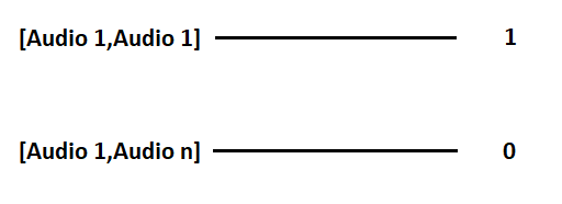
Here our Siamese neural network aims to find the similarity between the images of two audio clips. So in order to achieve it, we create a data pair as follows.
在这里,我们的暹罗神经网络旨在发现两个音频剪辑的图像之间的相似性。 因此,为了实现它,我们如下创建数据对。

When the generator is asked to generate a batch of images then that batch contains data in the fashion as shown above. Let the batch size be n then n/2 of the batch will contain a pair of similar images and their label will be 1 while remaining n//2 will have pair of different images labeled as 0.
当要求生成器生成一批图像时,则该批包含以上述方式显示的数据。 假设批次大小为n,则该批次的n / 2将包含一对相似的图像,它们的标签将为1,而其余n // 2将具有一对不同的图像标记为0。
The function different_label_index makes sure we get different pair by generating a different index for both images.
功能 different_label_index通过为两个图像生成不同的索引来确保获得不同的对。
The function load_img loads the mel spectrogram images and resizes them.
函数load_img 加载梅尔光谱图图像并调整其大小。
def different_label_index(X):
    idx1=0
    idx2=0
    while idx1==idx2:
        idx1=np.random.randint(0,len(X))
        idx2=np.random.randint(0,len(X))
    return idx1,idx2
def load_img(path):
  img=cv2.imread(path)
  img=cv2.cvtColor(img,cv2.COLOR_BGR2RGB)
  img=cv2.resize(img,(150,150))
  return img


def batch_generator(X,batch_size):
  while True:
    data=[np.zeros((batch_size,150,150,3)) for i in range(2)]
    tar=[np.zeros(batch_size,)]


    #Generating same pairs.
    for i in range(0,batch_size//2):
      idx1=np.random.randint(0,len(X))
      img1=load_img(X[idx1])
      img1=img1/255


      data[0][i,:,:,:]=img1
      data[1][i,:,:,:]=img1
      tar[0][i]=1


    #Generating different pairs.
    for k in range(batch_size//2,batch_size):
      idx1,idx2=different_label_index(X)
      img1=load_img(X[idx1])
      img1=img1/255
      img2=load_img(X[idx2])
      img2=img2/255


      data[0][k,:,:,:]=img1
      data[1][k,:,:,:]=img2
      tar[0][k]=0
    np.delete(data[0],np.where(~data[0].any(axis=1))[0], axis=0) #Remove the data points in case they have zero value.
    np.delete(data[1],np.where(~data[1].any(axis=1))[0], axis=0)
    yield data,tar
Having created all the functions of our need now let’s read the songs in our songs folder which is currently acting as our dataset and save their spectrograms.
创建了我们所需的所有功能之后,现在让我们在Songs文件夹中读取歌曲,该文件夹当前充当我们的数据集并保存其声谱图。
In the below code we read each song file one by one using the librosa library and we save the spectrogram of the whole track divided in 10s each. So, while the song is searched the user needs to have at least a recording of 10s.
在下面的代码中,我们使用librosa库逐个读取每个歌曲文件,然后将整个音轨的频谱图保存为10s。 因此,在搜索歌曲时,用户至少需要录制10秒。
In my case songs are located in D:/Songs/ folder.
就我而言,歌曲位于D:/ Songs /文件夹中。
songs_list=os.listdir('D:/Songs/') #Lists all the files in the folder.


#Read the songs,divide them into 10s segment,create spectrogram of them


charsets=string.ascii_letters


def get_random_name():
    name=''.join([random.choice(charsets) for _ in range(20)])
    name=name+str(np.random.randint(0,1000))
    return name


for song in songs_list:
    print(song)
    songfile,sr=librosa.load('D:/Songs/'+song)
    duration=librosa.get_duration(songfile,sr)
    prev=0
    for i in range(1,int((duration//10)+1)):
        if i==int((duration//10)):
            """Since we are dividing the song in 10s segment there might be case that after taking 10
            fragments also few more seconds are left so in this case extra becomes extra=extra+(10-extra)
            from the previous segment."""
            extra=int((int(duration)/10-int(int(duration)/10))*10)
            st=(sr*i*10)-(10-extra)
            end=st+10
            songfrag=np.copy(songfile[st:end])
        else:
            songfrag=np.copy(songfile[prev:(sr*i*10)])
        specname=get_random_name()
        create_spectrogram(songfrag,sr,'./Spectrograms/'+specname+'.png')
        prev=sr*i*10
This generates the spectrogram of all the audio segments and stores in spectrograms folder in the same working directory.
这将生成所有音频片段的频谱图,并将其存储在同一工作目录中的spectrograms文件夹中。
Now let’s train the Siamese network on those mel spectrogram images using early stopping and model checkpoint with train and test split of 75% and 25% respectively.
现在,让我们使用提早停止和模型检查点在这些梅尔光谱图图像上训练暹罗网络,训练和测试拆分分别为75%和25%。
batch_size=10
specfilelist=os.listdir('./Spectrograms/')
specfilelist=['./Spectrograms/'+filename for filename in specfilelist]
specfilelist=shuffle(specfilelist)


X_train=specfilelist[0:int(0.75*len(specfilelist))]
X_test=specfilelist[int(0.75*len(specfilelist)):]


es = EarlyStopping(monitor='val_loss', mode='min', verbose=1, patience=10, min_delta=0.0001)
mc = ModelCheckpoint('embdmodel.hdf5', monitor='val_loss', verbose=1, save_best_only=True, mode='min')
history=siamese_net.fit_generator(batch_generator(X_train,batch_size),steps_per_epoch=len(X_train)//batch_size,epochs=50,validation_data=batch_generator(X_test,batch_size),
                            validation_steps=len(X_test)//batch_size,callbacks=[es,mc],shuffle=True)
Now we have successfully trained our siamese net and its ready for checking our songs but there is a serious issue that running a siamese network every time on our spectrograms to check the similarity is a very time consuming and computationally expensive process. Neural networks are themselves very computationally expensive. Therefore in the next section, we will use this model’s weight and build another optimal network. We will also apply a trick which will drop the time complexity from O(n²) to O(n).
现在,我们已经成功地训练了暹罗网络并准备好检查歌曲,但是存在一个严重的问题,就是每次在频谱图上运行暹罗网络来检查相似性是一个非常耗时且计算昂贵的过程。 神经网络本身在计算上非常昂贵。 因此,在下一部分中,我们将使用此模型的权重并构建另一个最佳网络。 我们还将应用一个技巧,将时间复杂度从O(n²)降为O(n)。
使用该暹罗网络中的权重创建神经网络,从而优化搜索 (Creating a neural network using weights from this siamese network which optimizes the search)
Since the Siamese network will have to run every time the comparison is made that will prove to be a huge computation burden for our system. In this section, we propose the idea of distance estimation between the feature of the fragment of the song. So the neural network will have to run only once during the whole search process.
由于每次进行比较时都必须运行暹罗网络,因此对我们的系统来说,这将成为巨大的计算负担。 在本节中,我们提出了在歌曲片段特征之间进行距离估计的想法。 因此,神经网络在整个搜索过程中仅需运行一次。
The idea is that since the Siamese network shares the same weights between the networks, we can grab those weights and can create a single network having the same architecture as that of blocks N1 and N2 in our siamese network and transfer the weights from our previous network to it. The resulting network will be able to create embeddings of the fragments of the songs which are to be stored in our database. When the user queries a song the song is converted to embeddings stored in our database and the song which is having maximum similarity or minimum distance is returned.
这样的想法是,由于暹罗网络在网络之间共享相同的权重,因此我们可以抓住这些权重,并可以创建一个与暹罗网络中的N1和N2块具有相同架构的单个网络,并从先前的网络中转移权重对它。 由此产生的网络将能够创建要存储在我们数据库中的歌曲片段的嵌入。 当用户查询歌曲时,歌曲将转换为存储在我们数据库中的嵌入内容,并返回具有最大相似度或最小距离的歌曲。
Let me break the idea in subsequent steps.
让我在后续步骤中打破主意。
Let’s import all the libraries that we need. Also let’s borrow few helper functions from the previous sections.
让我们导入所需的所有库。 另外,让我们从前面的部分中借用一些辅助函数。
Note:-All these codes belong to another file called test.
注意:-所有这些代码属于另一个名为test的文件。
import os
from keras.models import load_model,Model
from keras.layers import Lambda,Dense,Input
import keras.backend as K
import librosa.display
import cv2
import librosa
import matplotlib.pyplot as plt
import librosa.display
import numpy as np
import string
import random


def create_spectrogram(clip,sample_rate,save_path):
  plt.interactive(False)
  fig=plt.figure(figsize=[0.72,0.72])
  ax=fig.add_subplot(111)
  ax.axes.get_xaxis().set_visible(False)
  ax.axes.get_yaxis().set_visible(False)
  ax.set_frame_on(False)
  S=librosa.feature.melspectrogram(y=clip,sr=sample_rate)
  librosa.display.specshow(librosa.power_to_db(S,ref=np.max))
  fig.savefig(save_path,dpi=400,bbox_inches='tight',pad_inches=0)
  plt.close()
  fig.clf()
  plt.close(fig)
  plt.close('all')
  del save_path,clip,sample_rate,fig,ax,S


def load_img(path):
  img=cv2.imread(path)
  img=cv2.cvtColor(img,cv2.COLOR_BGR2RGB)
  img=cv2.resize(img,(150,150))
  return img
Now let’s load the trained Siamese model and have a look at its representation in Keras using the summary function of the model class.
现在,让我们加载经过训练的暹罗模型,并使用模型类的摘要函数查看其在Keras中的表示形式。
model=load_model('embdmodel.hdf5')
model.summary()
Since the Siamese network shared the same weights across the block N1 and N2, then Keras uses the same layer for predicting both Vector 1 and Vector 2 which is evident from the model’s summary. Hence we can grab that layer from the Siamese model which will act as our new model for generating embedding.
由于暹罗网络在块N1和N2上共享相同的权重,因此Keras使用相同的层来预测Vector 1和Vector 2,这从模型的总结中可以明显看出。 因此,我们可以从Siamese模型中获取该层,该模型将用作生成嵌入的新模型。
Using model.layers attribute of the model class we can get the layers of the model as list. If we pay attention to the summary of the model we can observe that the layer we wanted is present as index 2. Hence we can get that layer as demonstrated below.Also we will look at the summary of this new model.
使用模型类的model.layers属性,我们可以获得列表的模型层。 如果我们关注模型的摘要,我们可以观察到我们想要的层以索引2的形式出现。因此,我们可以得到该层,如下所示。此外,我们还将查看这个新模型的摘要。
embedding_model=model.layers[2]
embedding_model.summary()
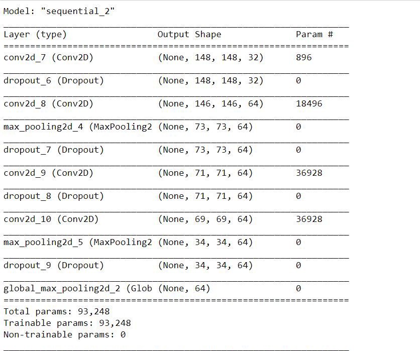
It is clear from the model’s summary that the new model has the same structure as the N1 or N2 block of the Siamese model and hence it can be used to generate embedding of the song’s fragment. Also since the model has been obtained from the trained Siamese model then it has all its weights.
从模型的摘要中可以明显看出,新模型与暹罗模型的N1或N2块具有相同的结构,因此可以用来生成歌曲片段的嵌入。 同样,由于该模型是从训练有素的暹罗模型中获得的,因此它具有所有权重。
Now same as the previous section where we created spectrograms for the fragments of the songs to train the model here also we will create a spectrogram and store them in another folder called Test_Spectrograms. Soon after we create the file using the create_spectrogram function, we will also open that file and will use the embedding model to generate embedding for it. Also at the same time, we add the name of the song we are processing as a key in dictionary songsspecdict. The value of the key is the array containing all the fragments embedding of that song.
现在与上一节中我们为歌曲的片段创建频谱图以在此处训练模型相同,我们还将创建一个频谱图并将其存储在另一个名为Test_Spectrograms的文件夹中。 在使用create_spectrogram函数创建文件后不久,我们还将打开该文件,并使用嵌入模型为其生成嵌入。 同时,我们将正在处理的歌曲的名称添加为字典songsspecdict中的键。 键的值是包含该歌曲所有嵌入片段的数组。
Here we are interested in the dictionSary obtained above. For the sake of simplicity, I decided to store the songs embedding in the dictionary instead of the database so that most of our readers understand it.
在这里,我们对上面获得的字典感兴趣。 为了简单起见,我决定将嵌入歌曲的歌曲而不是数据库存储在字典中,以便大多数读者都能理解。
Also after dictionary is created we save it using pickle library for later use.
同样,在创建字典后,我们使用泡菜库将其保存以备后用。
#Read the songs,divide them into 10s segment,create spectrogram of them


charsets=string.ascii_letters


songspecdict={}


songs_list=os.listdir('./test_songs/')


def get_random_name():
    name=''.join([random.choice(charsets) for _ in range(20)])
    name=name+str(np.random.randint(0,1000))
    return name


for song in songs_list:
    print(song)
    songfile,sr=librosa.load('./test_songs/'+song)
    duration=librosa.get_duration(songfile,sr)
    prev=0
    emblist=[]
    for i in range(1,int((duration//10)+1)):
        if i==int((duration//10)):
            extra=int((int(duration)/10-int(int(duration)/10))*10)
            st=(sr*i*10)-(10-extra)
            end=st+10
            songfrag=np.copy(songfile[st:end])
        else:
            songfrag=np.copy(songfile[prev:(sr*i*10)])
        specname=get_random_name()+'.png'
        create_spectrogram(songfrag,sr,'./Test_Spectrograms/'+specname)
        img_t=load_img('./Test_Spectrograms/'+specname)
        img_t=np.expand_dims(img_t,axis=0)
        emb=embedding_model.predict(img_t)
        emblist.append(emb)


        prev=sr*i*10
    songspecdict[song]=emblist


import pickle


with open('dict.pickle', 'wb') as handle:
    pickle.dump(songspecdict, handle, protocol=pickle.HIGHEST_PROTOCOL)
Our dictionary appears like this:-
我们的字典看起来像这样:
{‘song1’:[frag1_embedding,frag2_embedding,….fragN_embedding],’song2’:[frag1_embedding,frag2_embedding,….fragN_embedding],……}.
{'song1':[frag1_embedding,frag2_embedding,.... fragN_embedding],'song2':[frag1_embedding,frag2_embedding,.... fragN_embedding],……}。
Now let’s load the dictionary for searching.
现在,我们加载字典进行搜索。
import pickle
with open('dict.pickle', 'rb') as handle:
    songspecdict = pickle.load(handle)
Now we are all set for performing the search.
现在我们已经准备好执行搜索。
执行搜索 (Performing the search)
Here we will load the first 10 sec of the song the best day by Taylor Swift and we will create a spectrogram of it. We will then use our embedding model to generate embedding for it. This embedding will be compared with those stored in our dictionary and the one whose distance is minimum then its key will be returned as the title of the song.
在这里,我们将加载Taylor Swift最好的一天中歌曲的前10秒,并为其创建一个频谱图。 然后,我们将使用我们的嵌入模型为其生成嵌入。 此嵌入内容将与存储在我们词典中的嵌入内容进行比较,并且其距离最小,然后将其键作为歌曲的标题返回。
song,sr=librosa.load('test_songs/'+'18 The Best Day.m4a')
to_match=np.copy(song[0:220500])
create_spectrogram(to_match,22050,'test.png')
songsdistdict={}


to_match_img=load_img('test.png')
to_match_img=np.expand_dims(to_match_img,axis=0)


to_match_emb=embedding_model.predict(to_match_img)


for key,values in songspecdict.items():
    dist_array=[]
    for embd in values:
        dist_array.append(np.linalg.norm(to_match_emb-embd))

    songsdistdict[key]=min(dist_array)


song_titles=list(songsdistdict.keys())
distances=list(songsdistdict.values())


print(f'Recognized Song={song_titles[distances.index(min(distances))]}')
My test_songs folder contained the following songs:
我的test_songs文件夹包含以下歌曲:
13 Breathe (feat. Colbie Caillat).m4a
13 Breathe(feat。Colbie Caillat).m4a
14 Tell Me Why.m4a
14告诉我为什么
15 You’re Not Sorry.m4a
15你不抱歉.m4a
16 The Way I Loved You.m4a
16我爱你的方式.m4a
18 The Best Day.m4a
18最好的一天.m4a
Taylor Swift — Fearless — Mp3indir.ML.mp3.
泰勒·斯威夫特(Taylor Swift)—无所畏惧— Mp3indir.ML.mp3。
The output was:-
输出为:-

完善系统 (Improving the system)
Here as you can observe that we used the part of the original recorded track for searching but in the real world the recording may involve various noises in the background like vehicle horns, people talking, etc. Also, the first 10 sec of recording may or may not include the full content of which was supposed to be present in instead say we recorded from 2 sec after the song was played so this track alignment may not be present in a real-world case. Since I wanted to explain the concept in the most simple way so I created a very simple dataset since creating a full-fledged dataset alone is a very time-consuming task. I just created a dataset that was sufficient for explaining the concept.
在这里您可以看到,我们使用原始录制曲目的一部分进行搜索,但是在现实世界中,录制可能会在背景中涉及各种噪音,例如汽车喇叭,说话的人等。此外,录制的前10秒可能可能不会包含应该存在的全部内容,而是说我们是在播放歌曲后的2秒钟开始录制的,因此在实际情况下可能不会出现这种音轨对齐方式。 由于我想以最简单的方式解释该概念,所以我创建了一个非常简单的数据集,因为仅创建完整的数据集是一项非常耗时的任务。 我刚刚创建了一个足以解释该概念的数据集。
- A better dataset could be used which contains the recordings of the songs in various conditions. 可以使用更好的数据集,其中包含各种条件下歌曲的录音。
- Data augmentation could be done. 可以进行数据扩充。
- After obtaining a suitable dataset the model itself could be fine-tuned by adding more layers keeping the bias-variance tradeoff. 在获得合适的数据集之后,可以通过添加更多层以保持偏差方差折衷来对模型本身进行微调。
Congrats you have just learned how these music search systems work and you are in place to build your own. If you have some doubts regarding the above concepts feel free to leave down in the comment section.
恭喜,您已经了解了这些音乐搜索系统的工作原理,并且可以自行构建自己的音乐。 如果您对以上概念有疑问,请随时在评论部分中忽略。
Link to jupyter notebooks:-
链接到Jupyter笔记本:-
音乐雷达 shazam算法


 1413
1413

 被折叠的 条评论
为什么被折叠?


