客户流失预测_如何不预测和防止客户流失

客户流失预测

Customers are any business’ bread and butter. Whether it is a B2B business model or B2C, every company strives for a sticky customer base with minimal attrition to ensure an ongoing, recurring revenue stream.

客户是任何企业的生计。 无论是B2B商业模式还是B2C，每家公司都在努力争取粘性最小的客户群，以确保持续不断的经常性收入来源。

But how do you determine the specific customer characteristics that ensure customer longevity? How to identify ‘at-risk’ customers, i.e., those that are likely to churn? Given a customer’s probability to churn, just when can we expect him to churn? Important still, how much can we afford to invest in ‘at-risk’ customers to try and retain them?

但是，您如何确定确保客户寿命的特定客户特征？ 如何识别“高风险”客户，即那些可能流失的客户？ 考虑到客户流失的可能性，我们什么时候可以期望他流失？ 仍然重要的是，我们有多少钱可以投资于“高风险”客户以挽留他们？

These are all the questions that a business should ideally have answers to if it is interested in minimizing its customer churn. And I will try to help you get answers to these.

如果企业有兴趣最大程度地减少客户流失，那么所有这些都是企业理想的答案。 我会尽力帮助您获得这些答案。

Analyzing customer churn in a non-contractual setting (e.g., retail) is a non-trivial exercise since churn cannot be discretely defined here. A customer who has made X number of purchases so far can either return for another purchase, or may never return. Various approaches have been proposed to tackle this, including anomaly detection and Lifetime Value (LTV) analysis. I aim to cover LTV analysis in a non-contractual setting in my next post.

因为在这里不能单独定义客户流失，所以在非合同环境(例如零售)中分析客户流失并非易事。 迄今为止已完成X次购买的客户可以返回再进行一次购买，或者可能永远也不会返回。 已经提出了各种方法来解决此问题，包括异常检测和生命周期价值(LTV)分析。 我的下一篇文章旨在以非合同形式介绍LTV分析。

Contractual or subscription-based models, however, are easier to analyze since churn is a binary classification problem at a given point in time in these scenarios. If a customer does not renew his subscription, then he has undoubtedly churned. There can be no two ways about this: either a customer is active or has churned. We will cover churn analysis as applicable to subscription models in this post.

但是，基于合同或基于订阅的模型更易于分析，因为在这些情况下，流失是给定时间点的二进制分类问题。 如果客户不续订，那无疑是搅动了。 不可能有两种方法：客户是活跃的还是已经搅动了。 我们将在本文中介绍适用于订阅模型的客户流失分析。

Traditional approaches to churn modeling have utilized logistic regression, random forests, or gradient descent boosting to analyze and predict customer churn. However, we will utilize Survival Analysis techniques to gain additional insights related to customer churn. This will help us to answer the further questions stated at the beginning of this article.

传统的客户流失建模方法已经利用逻辑回归，随机森林或梯度下降提升来分析和预测客户流失。 但是，我们将利用生存分析技术来获得与客户流失相关的其他见解。 这将有助于我们回答本文开头提到的其他问题。

但是什么是生存分析？ (But What is Survival Analysis?)

Survival Analysis is a branch of statistical analysis, which addresses questions such as ‘how long would it be before a particular event occurs’, i.e., it is a ‘time to event’ model (compared to the probability of an event happening). Traditionally, survival analysis is heavily used in the medical and life sciences fields to determine the expected lifespan of an individual or other biological organisms.

生存分析是统计分析的一个分支，它解决诸如“在发生特定事件之前需要多长时间”之类的问题，即，它是“事件发生时间”模型(与事件发生的可能性相比)。 传统上，生存分析在医学和生命科学领域中大量使用，以确定个体或其他生物有机体的预期寿命。

Survival analysis is applicable in situations where we can define:

生存分析适用于以下情况：

• A ‘Birth’ event: for us, this will be a customer entering a contract with a company
  “出生”事件：对于我们来说，这将是与公司签订合同的客户
• A ‘Death’ event: for us, ‘death’ occurs when a customer does not renew its subscription
  “死亡”事件：对我们来说，“死亡”是指客户不续订订阅

While logistic regression and decision trees are appropriate for binary classification problems (will the customer churn or not?), Survival Analysis goes beyond that to answer when will the customer churn. If we do not expect a customer to churn right now, it does not automatically imply that he will never churn. If not now, there is a high probability that he might churn later. In such cases, survival analysis can throw light on such ‘censored’ customers by predicting their survival (or churn) at various points of time in the future.

尽管逻辑回归和决策树适用于二元分类问题(客户流失与否？)，但生存分析不仅仅可以回答客户流失的时间。 如果我们不希望客户现在就流失，那并不能自动暗示他永远也不会流失。 如果不是现在，那么他以后很可能流失。 在这种情况下，生存分析可以通过预测未来各个时间点的生存(或流失)来向这类“受审查”的客户提供启发。

This ability to deal with ‘censorship’ in data makes survival analysis a superior technique to other regression and tree-based models.

这种处理数据“审查”的能力使生存分析成为优于其他回归和基于树的模型的技术。

审查资料 (Censored Data)

In the traditional sense, censorship refers to losing track of an individual during an observation period, or where the event of interest is not observed during this period. This data is ‘censored’ because everyone dies or leaves/cancels a subscription at some future point in time; we’re just missing that information. Only because we haven’t observed them canceling their contact or subscription doesn’t mean they never will. And we can’t wait till they cancel their subscription to do our analysis. This is called Right-Censorship.

在传统意义上，检查是指在观察期内失去对某个人的跟踪，或者在此期间未观察到感兴趣的事件。 此数据被“审查”，因为每个人在某个将来的时间点都会死亡或退出/取消订阅。 我们只是缺少这些信息。 仅仅因为我们还没有观察到他们取消他们的联系或订阅，并不意味着他们永远不会。 我们迫不及待地希望他们取消订阅以进行分析。 这称为权利审查。

Other types of censorship include Left-Censorship and Interval-Censorship. The former refers to the scenario where we do not know when an individual became our customer because his ‘birth’ event happened before our observation time period. In contrast Interval-Censorship occurs when data is collected at specific time intervals that do not constitute a continuous observation period. Thereby, some life/death events could have missed out from being represented in the data.

其他类型的检查包括左检查和间隔检查。 前者是指这样的情况，即我们不知道某人何时成为我们的客户，因为他的“出生”事件发生在我们的观察时间段之前。 相反，当以特定时间间隔(不构成连续观察期)收集数据时，就会发生间隔检查。 因此，某些生/死事件可能会错过数据中的表示。

术语 (Terminologies)

• Time of Event: the time at which the event of interest occurs — churn or non-renewal of subscription in our case
  事件发生的时间：关注事件发生的时间-在我们的案例中，订阅流失或未续订
• Time of Origin: time at which a customer starts the service /subscription
  原始时间：客户启动服务/订阅的时间
• Time to Event: the difference between the Time of Event and the Time of Origin
  事件发生时间：事件发生时间与起源时间之间的时差

• Survival Function: This gives us the probability that our event of interest has not occurred by the time t. In other words, it provides us with the proportion of the population with the Time to Event value more than t

  生存函数：这使我们有机会在时间t没有发生我们感兴趣的事件。 换句话说，它为我们提供了事件发生时间值大于t的人口比例

• Hazard Function: This gives us the probability that our event of interest occurs at a specific time. Survival function can be derived from the Hazard function and vice versa
  危害功能：这使我们有可能在特定时间发生我们关注的事件。 生存功能可以从危害功能中得出，反之亦然
• Hazard Ratio is the ratio of the probability of our event of interest occurring for two different covariate groups (e.g., married or not). For example, a hazard ratio of 1.10 implies that the presence of a covariate increases the probability of risk event by 10%
  危害比率是我们感兴趣的事件在两个不同协变量组(例如已婚或未婚)中发生的概率的比率。 例如，危险比为1.10表示存在协变量会使风险事件的概率增加10％
• Covariates refer to predictors, variables or features in survival analysis
  协变量是指生存分析中的预测变量，变量或特征

Survival analysis techniques are designed to identify the survival function through two main data points: duration or Time to Event and a binary flag, whether our event of interest has occurred or not for each observation. Survival analysis is not really concerned with the Time of Event or Time of Origin. Instead, the Time to Event information is of paramount importance.

生存分析技术旨在通过两个主要数据点来识别生存功能：持续时间或事件发生时间以及二进制标记，无论我们的关注事件是否已针对每个观察发生。 生存分析与事件时间或起源时间无关。 相反，事件发生时间信息至关重要。

生存分析和信用风险分析 (Survival Analysis and Credit Risk Analysis)

Several studies have been conducted to determine if survival analysis can also predict both the probability and the expected time to the customer default However, no significant improvement was observed relative to traditional logistic regression methods. Plus, the fact that banking regulators and Basel accord require an easily comprehensible and interpretable methodology for credit decisions makes logistic regression a superior choice in these cases.

已经进行了一些研究来确定生存分析是否还可以预测到客户违约的可能性和预期时间。但是，相对于传统的逻辑回归方法，没有观察到明显的改善。 此外，银行业监管机构和巴塞尔协议要求信贷决策采用易于理解和可解释的方法，这一事实使得逻辑回归在这些情况下成为上乘之选。

生存/危险功能估计 (Survival/Hazard Function Estimation)

We will cover the two most well-established, documented, and in-practice models to estimate the survival and hazard functions through observed data.

我们将介绍两个最完善的，有据可查的和在实践中的模型，以通过观察到的数据估算生存和危害功能。

Kaplan-Meier(KM)生存分析 (Kaplan-Meier (KM) Survival Analysis)

Although we don’t have the true survival curve of the population, we can estimate a population’s survival function based on observed data through a powerful non-parametric method called the Kaplan-Meier estimator. The KM Survival Curve plots time on the x-axis and the estimated survival probability on the y-axis.

尽管我们没有人口的真实生存曲线，但是我们可以通过强大的非参数方法(称为Kaplan-Meier估计器)，根据观察到的数据来估计人口的生存函数。 KM生存曲线在x轴上绘制时间，在y轴上绘制估计的生存概率。

KM Survival Analysis requires only two inputs to predict the survival curve: Event (churned/non-churned) and Time to Event. Note that no other features or predictors are utilized by KM to assess the survival function.

KM生存分析仅需要两个输入来预测生存曲线：事件(搅动/非搅动)和事件发生时间。 注意，KM没有使用其他特征或预测变量来评估生存功能。

考克斯比例危害(CPH)模型 (Cox Proportional Hazard (CPH) Model)

In real-life situations, along with the event and duration data, we also have various other covariates (features or predictors) of the individuals in our population. It could very well be that these additional covariates also impact the probability of our event of interest not occurring (called survival probability) at a specific point in time in the future. For example, in a telco setting, these additional features could include gender, age, household size, monthly charges, etc. CPH model can handle both categorical and continuous covariates.

在现实生活中，连同事件和持续时间数据，我们还具有人口中个体的其他各种协变量(特征或预测变量)。 这些附加协变量也很可能也会影响我们感兴趣的事件在将来的特定时间点未发生的概率(称为生存概率)。 例如，在电信公司环境中，这些附加功能可能包括性别，年龄，家庭人数，每月费用等。CPH模型可以处理分类协变量和连续协变量。

The CPH model determines the effect that a unit change in a covariate will have on an observation’s survival probability. CPH is a semi-parametric model comprising of two parts:

CPH模型确定协变量的单位变化对观测值的生存概率的影响。 CPH是一个半参数模型，包含两个部分：

• The baseline hazard function being the non-parametric part of the model. Recall that the hazard function shows the risk or probability of an event occurring over future periods. The baseline hazard function estimates this risk at ‘baseline’ levels of covariates (usually mean values) and is generally similar to the KM Curve
  基线危害函数是模型的非参数部分。 回想一下，危害函数显示了将来发生事件的风险或概率。 基线风险函数在协变量的“基线”水平(通常是平均值)上估计此风险，并且通常类似于KM曲线
• The covariates’ relationship with the baseline hazard function, being the parametric part of the model. This relationship is represented as a time-invariant factor (or coefficient) that directly affects the baseline hazard.
  与基准风险函数的协变量关系，是模型的参数部分。 这种关系表示为直接影响基线危害的时不变因子(或系数)。

The real essence of a semiparametric model lies in the fact that it allows us to have the best of both worlds: a model that is interpretable and can be manipulated (parametric part) while still offering a fair representation of the real-life data without making any assumptions related to its functional form (non-parametric part).

半参数模型的真正本质在于，它使我们能够同时兼顾两个方面：一个可解释且可操纵的模型(参数部分)，同时仍能提供真实数据的公平表示而无需与功能形式有关的任何假设(非参数部分)。

However, the CPH model has a very strong assumption, called the proportional hazards assumption. This assumption states that a covariate’s associated hazard may change over time, but the hazard ratio remains constant over time. Consider the married binary covariate: the hazard or risk of a married individual dying may change over time. But the ratio of the following two is assumed to remain constant over time:

但是，CPH模型具有非常强的假设，称为比例风险假设。 该假设表明，协变量的相关风险可能随时间而变化，但是风险比率随时间保持不变。 考虑married二元协变量：已婚个体死亡的危险或风险可能会随时间变化。 但是，假定以下两个比率随时间保持不变：

• risk of a married individual dying at time t

  已婚人士在时间t死亡的风险

• risk of an unmarried individual dying at time t

  未婚个人在时间t死亡的风险

We will discuss this assumption in detail and whether any deviations can be tolerated in real-life applications during our practical example later in this post.

在本文后面的实际示例中，我们将详细讨论该假设，以及在实际应用中是否可以容忍任何偏差。

生存分析案例研究-客户保留率 (Survival Analysis Case Study — Customer Retention)

Enough with the theory, let us now turn to a practical case study where we will utilize Survival Analysis techniques on a telco customer data set to predict when specific customers are expected to churn and how much we can afford to spend to retain them.

有了足够的理论，现在让我们转到一个实际的案例研究中，我们将在电信公司客户数据集上使用生存分析技术，以预测特定客户何时会流失，以及我们有多少能力花钱保留他们。

All the related survival analysis techniques are included in the lifelines package available for Python. We will use a publicly available dataset of telco customers containing, among other covariates, information on an individual’s tenure/duration with the company together with a binary flag representing whether he has churned or not as at the date of data collection:

所有相关的生存分析技术都包含在可用于Python的lifelines包中。 我们将使用电信客户的公开数据集 ，其中除其他协变量外，还包含有关个人与公司的任期/任期的信息，以及代表他在数据收集之日是否曾进行过搅动的二进制标志：

Our initial data exploration reveals the following:

我们的初步数据探索显示以下内容：

• All but one covariate are of object datatype, implying that we need one-hot encode them

  除一个协变量外，其他所有变量都是object数据类型，这意味着我们需要对其进行一键编码

• TotalCharges is of an object datatype instead of being float64. The reason appears to be some white spaces for specific observations

  TotalCharges具有object数据类型，而不是float64 。 原因似乎是某些空格用于特定观察

• Unique identifiers (customerID in this case) are usually dropped for model training. However, our end objective here is also to identify and plan customer level strategies to reduce the churn of our currently non-churned customers. Therefore, we will carve out the customerID & MonthlyCharges of active and censored individuals into a separate dataframe to be used later on when designing customer level strategies

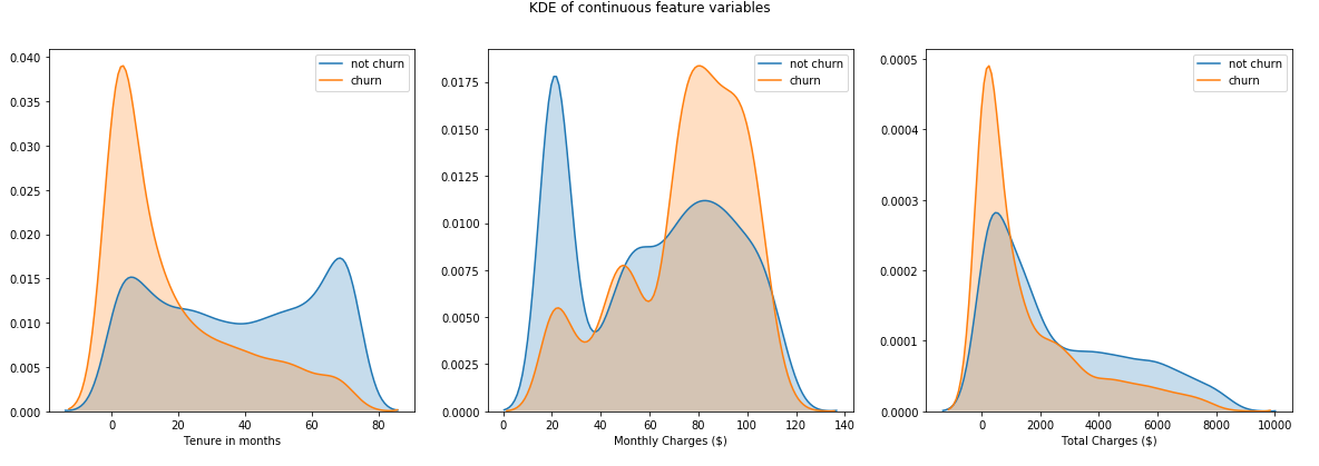
  通常会删除唯一标识符(在这种情况下为customerID )以进行模型训练。 但是，我们的最终目标还是要确定和计划客户级别的策略，以减少我们目前未流失的客户的流失率。 因此，我们将把活跃的和被检查的个人的customerID MonthlyCharges和每月费用划分为一个单独的数据框，以便以后在设计客户级别策略时使用

• KDE plots of continuous variables depict skewed distributions
  连续变量的KDE图描述了偏斜分布

We will then perform the following feature engineering steps to prepare our data for survival analysis:

然后，我们将执行以下功能工程步骤，以准备用于生存分析的数据：

• Replace the white space in TotalCharges with the value of the MonthlyCharges column and convert it to a numeric datatype.

  将TotalCharges的空白替换为MonthlyCharges列的值，并将其转换为数字数据类型。

• Replace Yes and No values of our target Churn column with 1 and 0, respectively.

  分别将目标Churn列的Yes和No值替换为1和0。

• Similarly, for other specific features, replace Yes with 1 and 0 for other values (e.g., No, No internet service).
  同样，对于其他特定功能，将“是”替换为1，将其他值替换为0(例如，“否”，“否”互联网服务)。
• Create dummy variables of the remaining categorical features.
  创建其余分类特征的伪变量。

Note: For each dummy variable, we typically drop one of the encoded features to eliminate the risk of multicollinearity. However, we will manually drop a specific dummy variable that is generally representative of our subscriber population. When we drop one of our dummy columns, the value of that dropped column becomes represented in the baseline hazard function. Manually controlling which dummy variable should be dropped ensures that our baseline hazard function is representative of a typical subscriber. Everything else is a deviation away from this recognized baseline, thereby being intuitively understood by the business. Therefore, we will drop that dummy variable that occurs most frequently in our sample.

注意 ：对于每个虚拟变量，我们通常会删除其中一个编码特征，以消除多重共线性的风险。 但是，我们将手动删除一个特定的虚拟变量，该变量通常代表我们的订户总数。 当我们删除其中一个虚拟列时，该删除列的值将在基线危害函数中表示。 手动控制应删除哪个虚拟变量可确保我们的基线危险函数代表典型的订户。 其他所有内容均偏离此公认基准，因此企业可以直观地理解。 因此，我们将删除样本中最常出现的虚拟变量。

The CPH model implementation in lifelines does not work well with highly collinear covariates, so let’s check for the existence of multicollinearity through a heatmap:

生命线中的CPH模型实现不适用于高度共线性的协变量，因此让我们通过热图检查是否存在多重共线性：

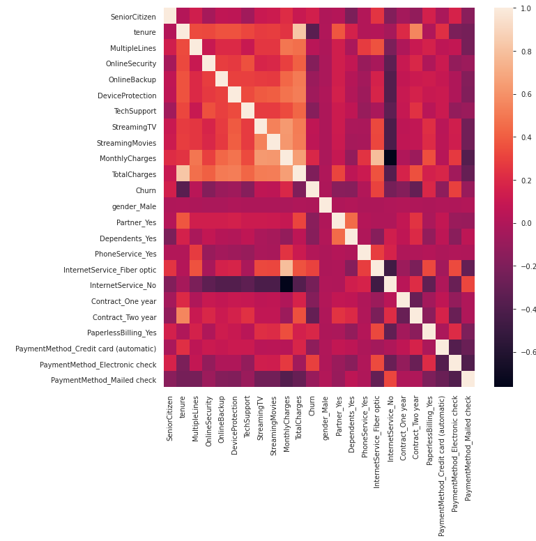
Since the above heatmap does not indicate any high pair-wise correlation, we will continue with our survival analysis.

由于上面的热图没有表明任何高的成对相关性，因此我们将继续进行生存分析。

Code for steps performed so far, other than that for visualizations and data exploration follows:

除了用于可视化和数据探索的代码外，还包括到目前为止执行的步骤的代码：

# Importing and installing all the required libraries
import pandas as pd
import numpy as np
import matplotlib.pyplot as plt
import seaborn as sns
from sklearn.calibration import calibration_curve 
from sklearn.metrics import brier_score_loss
! pip install lifelines==0.25.2
import lifelines


# Load data
data = pd.read_csv('.../churn_data.csv')


# Replace single white space with MonthlyCharges and convert to numeric
data['TotalCharges'] = data['TotalCharges'].replace(' ', data['MonthlyCharges']) 
data['TotalCharges'] = pd.to_numeric(data['TotalCharges'])


# Save customerID and MonthlyCharges columns in a separate DF and drop customerID from the main DF
churned_customers = data[data['Churn'] == 'No']
customerID = pd.DataFrame(churned_customers[['customerID', 'MonthlyCharges']])
data.drop(columns = ['customerID'], inplace=True)


# We will also create a copy of DF that will be utilised later to plot categorical KM Curves
data_kmf = data.copy()


# Convert Churn column to 1 (Yes) or 0 (No)
data['Churn'] = data['Churn'].replace({"No": 0, "Yes": 1})


# Create a list of features where we will assign 1 to a Yes value and 0 otherwise
features_to_combine = ['MultipleLines', 'OnlineSecurity', 'OnlineBackup', 'DeviceProtection',
					   'TechSupport', 'StreamingTV', 'StreamingMovies']
# Assign 1 to Yes and 0 otherwise
for feat in features_to_combine:
    data[feat] = data[feat].apply(lambda x: 1 if x == 'Yes' else 0)


# Create dummy variables for our remaining categorical columns
data = pd.get_dummies(data, columns = ['gender', 'Partner', 'Dependents', 'PhoneService',
				       'InternetService', 'Contract', 'PaperlessBilling',
				       'PaymentMethod'], drop_first = False)
# Drop that dummy variable that the business considers to be typical of their subscribers
data.drop(columns = ['gender_Male', 'Partner_Yes', 'Dependents_No', 'PhoneService_Yes',
		     'InternetService_Fiber optic', 'Contract_Month-to-month', 'PaperlessBilling_Yes',
		     'PaymentMethod_Electronic check'], inplace = True)

Note: We are lucky here in the sense that our data already has a duration or tenure column. Oftentimes, instead of having these durations, you may encounter start and end times of each observation. lifelines has a handy utility function to convert start and end dates into a NumPy array of floats representing durations and a boolean array of event observations: datetimes_to_durations

注意 ：在这里我们很幸运，因为我们的数据已经具有持续时间或任期列。 通常，您可能会遇到每个观察的开始和结束时间，而不是具有这些持续时间。 lifelines具有方便的实用程序功能，可将开始日期和结束日期转换为代表持续时间的NumPy浮点数组和事件观察值的布尔数组： datetimes_to_durations

KM曲线 (KM Curve)

We will start our survival analysis by first plotting a KM curve of our sample that shows us the historical survival probability of an average customer at specific points in time. Remember that the presence of covariates has no impact on a KM curve as it is only concerned with the durations and an event flag. Usually, in practice, KM curves are looked at first to get a feel of our data before a more in-depth analysis through the CPH model.

我们将通过首先绘制样本的KM曲线开始我们的生存分析，该KM曲线向我们显示平均客户在特定时间点的历史生存概率。 请记住，协变量的存在对KM曲线没有影响，因为它仅与持续时间和事件标志有关。 通常，实际上，在通过CPH模型进行更深入的分析之前，首先要查看KM曲线以了解我们的数据。

Our first KM curve for all customers and with a 5% confidence interval looks something like this:

我们针对所有客户的第一个KM曲线，置信区间为5％，如下所示：

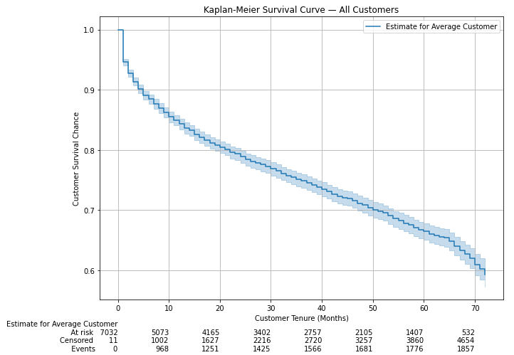
The above should give us some basic intuition about our customers. As we would expect for a telecom business, churn is relatively low. Even after 72 months (the max tenure in our data), the company can retain ~60% or more of its customers.

以上内容应使我们对客户有所了解。 正如我们对电信业务的预期，客户流失率相对较低。 即使在72个月后(我们数据中的最大任期)，该公司仍可以保留约60％或更多的客户。

The rows at the bottom of the plot shows some additional information to be interpreted as follows:

图表底部的各行显示了一些其他信息，如下所述：

• At-risk: number of customers with an observed tenure of more than the point in time. For example, 532 customers had a tenure of more than 70 months
  处于风险中：观察到的使用期限超过时间点的客户数量。 例如，有532位客户的任期超过70个月
• Censored: number of customers with a tenure equal to or less than the point in time, which were not churned. For example, 3,860 customers had a tenure of 60 months or less However, they had not churned then
  已审查：任期等于或小于时间点但未被搅动的客户数量。 例如，有3,860位客户的任期为60个月或更短，但是那时他们并没有进行培训
• Events: number of customers with a tenure equal to or less than the point in time, which had churned by then. For example, 1,681 customers had a tenure of 50 months or less and had churned by then
  事件：届满时任期等于或小于时间点的客户数量。 例如，有1,681位客户的任期为50个月或更短，并且到那时为止

At this point, we do not know which of our covariates have a material impact on our customer’s survival chances (the CPH model will help us with that). However, intuitively we know that having a more extended fixed-term contract can be expected to affect a customer’s survival probability. To examine this potential impact, we will draw KM curves for each unique value of the Contract column:

在这一点上，我们不知道哪个协变量会对客户的生存机会产生重大影响(CPH模型将帮助我们实现这一目标)。 但是，从直觉上讲，我们知道可以延长合同期限来影响客户的生存概率。 为了检查这种潜在影响，我们将为“合同”列的每个唯一值绘制KM曲线：

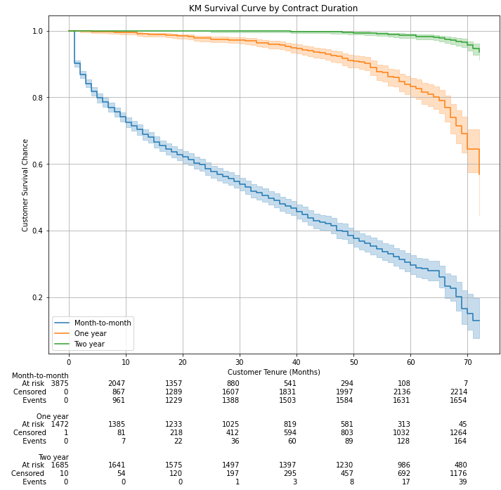
Materially different survival curves we have here with survival probabilities dropping sharply over time for customers on a monthly contract, as expected. Even after three years (at 40 months, to be precise):

正如我们所期望的，我们这里的月度合同的客户的生存概率会随着时间的推移而急剧下降，生存曲线大不相同。 即使在三年后(准确地说是40个月)：

• Customers on a 2 years contract have almost 100% survival probability
  签订2年合同的客户的生存几率几乎为100％
• Customers on a 1-year contract have more than 95% survival probability
  签订1年合同的客户的生存率超过95％
• Customers on a monthly contract have around only 45% survival probability
  签订月度合同的客户存活率只有约45％

# Instantiate KMF class with the default 5% CI, can be changed bthrough the alpha parameter
kmf = lifelines.KaplanMeierFitter()


# Fit KMF to our data
kmf.fit(durations = data['tenure'], event_observed = data['Churn'], 
        label = 'Estimate for Average Customer')


# Plot KM curve
fig, ax = plt.subplots(figsize = (10,7))
kmf.plot(at_risk_counts = True, ax=ax)
ax.set_title('Kaplan-Meier Survival Curve — All Customers')
ax.set_xlabel('Customer Tenure (Months)')
ax.set_ylabel('Customer Survival Chance')
ax.grid();


# Plot KM Curve for each category of 'Contract' column
# Update Churn column of data_kmf that we kept aside for this moment before feature engineering
data_kmf['Churn'] = data_kmf['Churn'].replace({"No": 0, "Yes": 1})


# save row indices for each contract type
idx_m2m = data_kmf['Contract'] == 'Month-to-month'
idx_1y = data_kmf['Contract'] == 'One year'
idx_2y = data_kmf['Contract'] == 'Two year'


# plot the 3 KM plots for each category
fig, ax = plt.subplots(nrows = 1, ncols = 1, figsize = (10,10))
kmf_m2m = lifelines.KaplanMeierFitter()
ax = kmf_m2m.fit(durations = data_kmf.loc[idx_m2m, 'tenure'], 
                 event_observed = data_kmf.loc[idx_m2m, 'Churn'],
                 label = 'Month-to-month').plot(ax = ax)
kmf_1y = lifelines.KaplanMeierFitter()
ax = kmf_1y.fit(durations = data_kmf.loc[idx_1y, 'tenure'],
                event_observed = data_kmf.loc[idx_1y, 'Churn'],
                label = 'One year').plot(ax = ax)
kmf_2y = lifelines.KaplanMeierFitter()
ax = kmf_2y.fit(durations = data_kmf.loc[idx_2y, 'tenure'],
                event_observed = data_kmf.loc[idx_2y, 'Churn'],
                label = 'Two year').plot(ax = ax)


# display title and labels
ax.set_title('KM Survival Curve by Contract Duration')
ax.set_xlabel('Customer Tenure (Months)')
ax.set_ylabel('Customer Survival Chance')
plt.grid()


# display at-risk counts for each category
lifelines.plotting.add_at_risk_counts(kmf_m2m, kmf_1y, kmf_2y, ax=ax);

CPH模型 (CPH Model)

Now comes the more interesting stuff where we will analyze the interaction between survival curves and other covariates in our data. Fitting a CPH model is just like any other ML model in scikit-learn. The following model summary is accessed through the model’s print_summary method:

现在出现了更有趣的内容，我们将分析生存曲线与数据中其他协变量之间的相互作用。 拟合CPH模型就像scikit-learn中的其他任何ML模型一样。 通过模型的print_summary方法可以访问以下模型摘要：

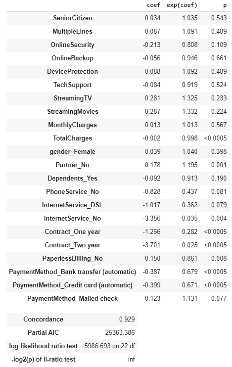
The above model summary lists down all of the one-hot encoded covariates analyzed by the CPH model. Let us look at the critical information presented here:

上面的模型摘要列出了CPH模型分析的所有一键编码的协变量。 让我们看看这里提供的关键信息：

• Model coefficients (coef column) tell us how each covariate impacts risk. A positive coef for a covariate indicates that a customer with that feature is more likely to churn and vice versa

  模型系数( coef列)告诉我们每个协变量如何影响风险。 协变量的正coef表示具有该功能的客户更容易流失，反之亦然

• exp(coef) is the hazard ratio, interpreted as the scaling of hazard risk for each additional unit of the variable, with 1.00 being neutral. For example, the 1.332 hazard ratio for StreamingMovies means a customer who is subscribed to a streaming movie service is 33.2% more likely to cancel their service. From our perspective, exp(coef) below 1.0 is good, meaning a customer is less likely to cancel in the presence of that covariate

  exp(coef)是危险比，解释为变量的每个其他单位的危险风险标度，其中1.00为中性。 例如， StreamingMovies的1.332危险比意味着订阅流电影服务的客户取消服务的可能性高33.2％。 从我们的角度来看， exp(coef)小于1.0是好的，这意味着在存在该协变量的情况下，客户取消交易的可能性较小

• Model Concordance of 0.929 is interpreted similarly to a logistic regression’s AUROC:

  模型一致性0.929的解释类似于逻辑回归的AUROC：

  — 0.5 is the expected result from a random prediction

  — 0.5是随机预测的预期结果

  — closer to 1.0, the better with 1.0 showing a perfect predictive concordance.

  —接近1.0，则1.0更好，表现出完美的预测一致性。

So our model’s concordance of 0.929 is a pretty good one!

因此，我们模型的0.929一致性非常好！

But what is the Concordance Index?

但是什么是一致性指数？

A Concordance of 0.929 basically means that our model correctly predicted 92.9 pairs out of 100 on uncensored data. It basically assesses the discriminatory power of a model, i.e., how good is it in differentiating between alive and churned subjects. It is useful to compare two different models. However, concordance does not say anything about how well our model is calibrated — something that we will evaluate later on.

0.929的一致性基本上意味着我们的模型在未审查的数据中正确预测了100 组中的92.9 对 。 它基本上评估了模型的区分能力，即，它在区分活着的和搅动的对象方面有多好。 比较两个不同的模型很有用。 但是，一致性并没有说明模型的校准程度，这将在以后进行评估。

A pair here refers to all the possible customer pairs in our data. Consider an example where we have five uncensored customers: A, B, C, D & E. From these five customers, we can have a total of ten possible pairs: (A, B), (A, C), (A, D), (A, E), (B, C), (B, D), (B, E), (C, D), (C, E) and (D, E). In case E is censored, then the Concordance Index calculation will exclude pairs related to E and will consider the remaining eight pairs in the denominator.

这里的一对是指数据中所有可能的客户对。 考虑一个例子，我们有五个未经审查的客户：A，B，C，D和E。从这五个客户中，我们总共可以有十对可能的对：(A，B)，(A，C)，(A， D)，(A，E)，(B，C)，(B，D)，(B，E)，(C，D)，(C，E)和(D，E)。 如果检查了E，则Concordance Index计算将排除与E相关的对，并考虑分母中其余的8对。

确认比例危害(PH)假设 (Confirm Proportional Hazards (PH) Assumption)

Recall the CPH model’s proportional hazards assumption that was explained above. The PH assumption can be checked using statistical tests and graphical diagnostics based on the scaled Schoenfeld residuals. The assumption is supported by a non-significant relationship between residuals and time (e.g., p > 0.05), and refuted by a significant relationship (e.g., p < 0.05).

回顾上面解释的CPH模型的比例风险假设。 可以根据缩放后的Schoenfeld残差使用统计测试和图形诊断来检查PH假设。 该假设得到残差与时间之间非显着关系的支持(例如，p> 0.05)，而被显着关系(例如，p <0.05)所推翻。

Without going into many technical details, I will instead focus on practical applications only. The PH assumptions can be checked by lifelines’ check_assumptions method on a fitted CPH model. Executing this method will return the names of the covariates that do not satisfy the PH assumption, some generic advice on how to rectify the PH violation potentially, and, for each variable that violates the PH assumption, visual plots of the scaled Schoenfeld residuals against time transformations (a flat line confirms PH assumption). Refer to this for further details.

在不涉及许多技术细节的情况下，我将只关注实际应用。 可以通过lifelines “ check_assumptions方法在拟合的CPH模型上检查PH假设。 执行此方法将返回不满足PH假设的协变量的名称，有关如何可能纠正PH违规的一些一般性建议，并且对于每个违反PH假设的变量，将按比例绘制Schoenfeld残差随时间变化的视觉图转换(一条平线确认PH假设)。 有关更多详细信息，请参考此内容。

Upon checking the PH assumption for our model, we find that 3 of our covariates do not conform to it. However, project’s purpose, we will ignore these warnings since our end objective is survival prediction and not to determine inference or correlation to understand the influence of a covariate on the survival duration and outcome. Refer to this for further details as to why we can safely ignore these deviations.

在检查了模型的PH假设后，我们发现3个协变量不符合该假设。 但是，出于项目目的，我们将忽略这些警告，因为我们的最终目标是生存预测，而不是确定推断或相关性以了解协变量对生存期和结果的影响。 有关我们为什么可以安全地忽略这些偏差的更多详细信息，请参考此内容。

CPH模型验证 (CPH Model Validation)

lifelines library has a built-in function to perform k-fold cross-validation of our fitted model. Running it using the concordance index as the scoring parameter results in an average concordance index of 0.928 across ten folds.

lifelines库具有内置功能，可以对我们的拟合模型执行k倍交叉验证。 使用一致指数作为评分参数运行它会得到10折的0.928的平均一致指数。

The Concordance Index does not say anything about the model’s calibration — i.e., how far are the predicted probabilities from the actual true probabilities? We can draw a calibration curve to check this propensity of our model to predict probabilities at any given time correctly. Let us now plot a calibration curve at t = 12 using sklearn’s calibration_curve function:

一致性指数没有说明模型的校准，即预测的概率与实际的真实概率有多远？ 我们可以绘制一条校准曲线来检查模型的这种倾向，以正确预测任何给定时间的概率。 现在让我们使用sklearn的calibration_curve函数在t = 12处绘制一条校准曲线：

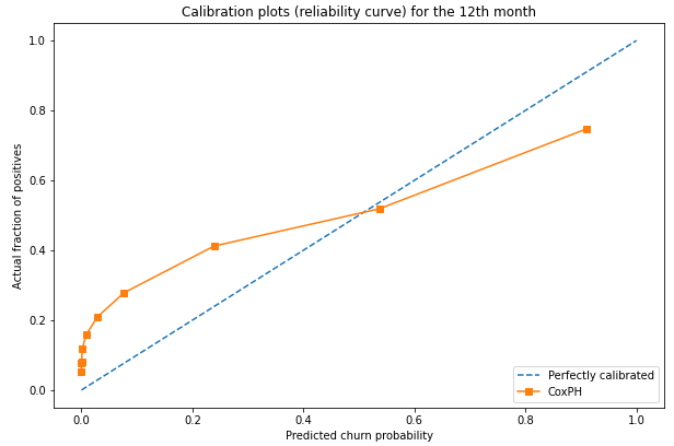
Given our data’s skewed distribution between churned and non-churned customers, we have set calibration_curve’s strategy parameter to ‘quantile’. This will ensure that each bin will have the same number of samples based on the predicted churn probabilities for the 12th month. This is desirable as otherwise, we would have equal width bins that would not be representative given the unbalanced class distribution between churned/non-churned customers.

鉴于我们的数据在搅动客户和非搅动客户之间的分布偏斜，我们已将calibration_curve的strategy参数设置为'quantile' 。 这将确保根据第12个月的预测流失概率，每个垃圾箱将具有相同数量的样本。 这是合乎需要的，否则，考虑到搅动/非搅动客户之间的类别分布不平衡，我们将具有相等宽度的分箱，这将不具有代表性。

The above calibration plot shows us that for the first seven deciles plotted, our CPH model under-predicted the churn risk and overpredicted for the last two.

上面的校准图显示，对于绘制的前七个十分位数，我们的CPH模型低估了流失风险，而高估了后两个风险。

Overall, the calibration curve doesn’t look too bad. Let’s confirm it by calculating the Brier Score, which we find to be 0.17 (0 is an ideal Brier Score), not bad at all!

总的来说，校准曲线看起来还不错。 让我们通过计算Brier分数来确认这一点，我们发现其为0.17(0是理想的Brier分数)，一点也不差！

We can also plot the Brier Score for each month, as follows:

我们还可以绘制每个月的Brier分数，如下所示：

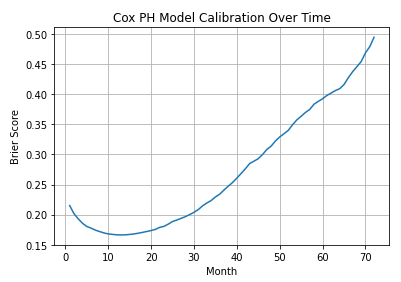
We can see that our model is reasonable calibrated between 5 and ~20 months and then deteriorates as we start to predict further out in time.

我们可以看到我们的模型在5到20个月之间进行了合理的校准，然后随着我们开始进一步预测时间而逐渐恶化。

CPH模型可视化 (CPH Model Visualization)

Let us now visualize the coefficients and hazard ratios of all the covariates analyzed in the CPH model:

现在让我们可视化CPH模型中分析的所有协变量的系数和风险比：

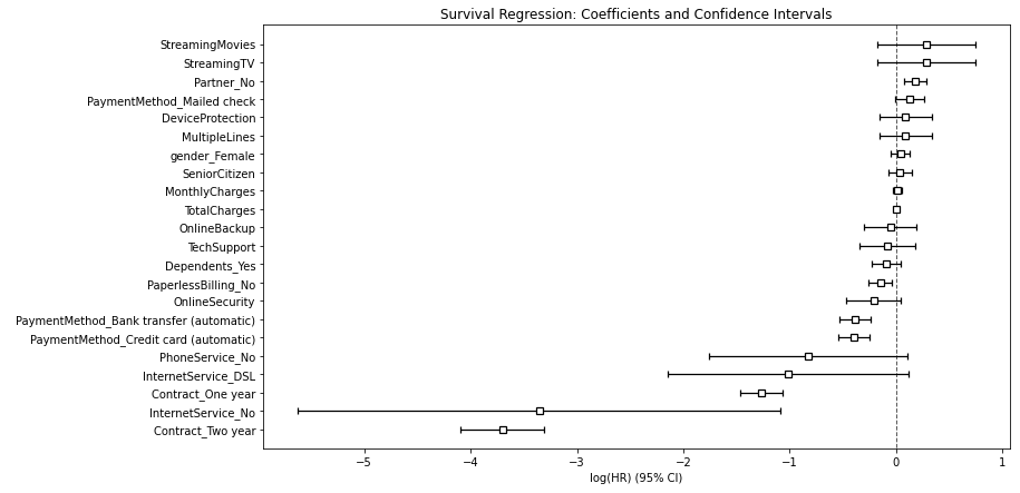
Through this plot, we can quickly identify the specific customer characteristics that are critical to predicting churn.

通过此图，我们可以快速确定对于预测客户流失至关重要的特定客户特征。

Covariates likely to result in churn:

可能导致客户流失的协变量：

• Streaming TV and Movies subscriptions
  流媒体电视和电影订阅
• Multiple phone lines
  多条电话线
• Device protection subscription
  设备保护订阅
• Individuals living alone
  个人独居
• Payments by mailed cheques
  通过邮寄支票付款

Covariates likely to help with customer retention:

可能有助于保留客户的协变量：

• Having a 1 or 2-year contract term (pretty obvious)
  具有1年或2年的合同期限(非常明显)
• Automatic payment methods
  自动付款方式
• No internet and phone services
  没有互联网和电话服务
• DSL internet service
  DSL上网服务

Let us now plot and visualize the effect of varying a covariate over the survival curve at specified levels together with the baseline survival curve:

现在，让我们绘制和可视化在指定水平上随生存曲线变化的协变量以及基线生存曲线的效果：

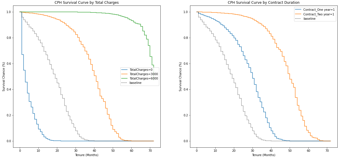
Evident that customers whose total spend is closer to zero are more at-risk (their survival curve drops off sharply) than those whose total spend is closer to 3,000 or more. Further, having a long-term contract improves the customer’s survival probability.

显而易见，总支出接近零的客户比总支出接近3,000或更高的客户更有风险(生存曲线急剧下降)。 此外，签订长期合同可以提高客户的生存率。

All the code related to CPH modeling, validation, visualization is below:

与CPH建模，验证，可视化相关的所有代码如下：

# Instantiate and fit CPH model
cph = lifelines.CoxPHFitter()
cph.fit(data, duration_col = 'tenure', event_col = 'Churn')


# Print model summary
cph.print_summary(model = 'base model', decimals = 3, columns = ['coef', 'exp(coef)', 'p']) 


# Check model assumptions, with a threshold of 0.001
cph.check_assumptions(data, p_value_threshold=0.001, show_plots=True)


# CPH MODEL VALIDATION
# Calculate the average Concordance Index across 10 folds
avg_score = np.mean(lifelines.utils.k_fold_cross_validation(cph, data, 'tenure',
							    'Churn', k = 10,
							    scoring_method = 'concordance_index'))
print('The average Concordance Score across 10 folds is: {:.3f}'.format(avg_score))


# Plot calibration curve at t=12
plt.figure(figsize=(10, 10))
ax1 = plt.subplot2grid((3, 1), (0, 0), rowspan=2) 
# Plot the perfectly calibrated line with 0 intercept and 1 slope
ax1.plot([0, 1], [0, 1], ls = '--', label = 'Perfectly calibrated') 
# Calculate the "churn" probabilities at the end of 12th month
probs = 1 - np.array(cph.predict_survival_function(data, times = 12).T)
actual = data['Churn'] 
# get the info required to plot a calibration curve for 10 deciles
fraction_of_positives, mean_predicted_value = calibration_curve(actual, probs, n_bins = 10, strategy = 'quantile') 
ax1.plot(mean_predicted_value, fraction_of_positives, marker = 's', ls = '-', label='CoxPH') 
ax1.set_ylabel("Actual fraction of positives") 
ax1.set_xlabel("Predicted churn probability")
ax1.set_ylim([-0.05, 1.05]) 
ax1.legend(loc="lower right") 
ax1.set_title('Calibration plots (reliability curve) for the 12th month');


# calculate Brier Score
brier_score = brier_score_loss(data['Churn'], 1 - np.array(cph.predict_survival_function(
	data, times = 12).T), pos_label = 1)
print('The Brier Score of our CPH Model is {:.2f} at the end of 12 months'.format(brier_score))


# plot brier score for the next 72 months
brier_score_dict = {} 
# Loop over all the months
for i in range(1,73): 
    score = brier_score_loss(data['Churn'], 1 - np.array(cph.predict_survival_function(data, times = i).T), pos_label=1) 
    brier_score_dict[i] = [score] 
# Convert the dict to a DF
brier_score_df = pd.DataFrame(brier_score_dict).T 
# Plot the Brier Score over time
fig, ax = plt.subplots() 
ax.plot(brier_score_df.index, brier_score_df) 
ax.set(xlabel='Month', ylabel='Brier Score', title='Cox PH Model Calibration Over Time') 
ax.grid()


# CPH MODEL VISUALIZATION
# plot CPH model coefficients and their respective confidence intervals
fig_coef, ax_coef = plt.subplots(figsize = (12,7))
ax_coef.set_title('Survival Regression: Coefficients and Confidence Intervals')
cph.plot(ax = ax_coef);


# plot CPH survival curves over various covariate values
fig, (ax1, ax2) = plt.subplots(nrows = 1, ncols = 2, figsize = (20,9))
# Total Charges
cph.plot_partial_effects_on_outcome('TotalCharges', values = [0, 3000, 6000], ax = ax1)
ax1.set_title('CPH Survival Curve by Total Charges')
ax1.set_xlabel('Tenure (Months)')
ax1.set_ylabel('Survival Chance (%)')
# Contract
cph.plot_partial_effects_on_outcome(['Contract_One year', 'Contract_Two year'], 
				    values = [[1, 0], [0, 1]], ax = ax2)
ax2.set_title('CPH Survival Curve by Contract Duration')
ax2.set_xlabel('Tenure (Months)')
ax2.set_ylabel('Survival Chance (%)');

流失预测与预防 (Churn Prediction and Prevention)

So now we know which covariates we can focus on to reduce the churn risk of our existing right-censored customers, i.e., those that have not churned yet. Let us first plot the categorical KM curves for Contract, PaymentMethod, InternetService, and PhoneService:

因此，现在我们知道可以集中精力处理哪些协变量，以减少我们现有的经过权利审查的客户(即那些尚未搅动的客户)的流失风险。 让我们首先绘制Contract ， PaymentMethod ， InternetService和PhoneService的分类KM曲线：

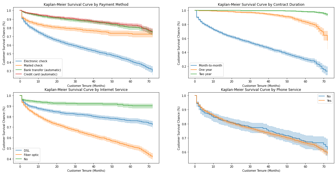
Insights:

见解：

• Encourage customers to set up automatic payments either through a bank transfer or credit card
  鼓励客户通过银行转帐或信用卡设置自动付款
• Pretty clear cut to have the customers on a 1 or 2-year contract
  很清楚，让客户签订1年或2年合同
• Regarding internet services, first of all, we should analyze the root cause of a relatively high customer churn who have either a DSL or Fiber Optic internet subscription — may be poor service quality, high prices, inadequate customer service, etc. We should also do a profitability analysis of internet services. The best course of action would depend on that analysis
  关于互联网服务，首先，我们应该分析客户流失率较高的根本原因，这些客户具有DSL或光纤互联网订阅-服务质量差，价格高，客户服务不足等。我们也应该这样做互联网服务的盈利能力分析。 最佳行动方案取决于该分析
• There does not appear to be much statistical difference in the survival curves of customers with or without a phone service
  有或没有电话服务的客户的生存曲线似乎没有太大的统计差异

分析被审查的客户 (Analyze Censored Customers)

Now we will turn our focus on censored and still alive customers to determine the future month in which they can be expected to churn together with what we do to increase their retention chances.

现在，我们将重点放在受审查并仍然存在的客户上，以确定可以预期他们在未来几个月内流失的机会以及我们为增加客户保留机会所做的工作。

After filtering our data for all customers where Churn == 0, we will use the predict_survival_function method to predict future survival curves of these customers given their respective covariates. That is, estimate the remaining life of our customers.

在过滤掉Churn == 0所有客户的数据之后，我们将使用predict_survival_function方法来预测这些客户在各自协变量下的未来生存曲线。 也就是说，估计客户的剩余寿命。

predict_survival_function’s output will be a matrix containing survival probability for each remaining customer at specific future points in time up to the maximum historical duration in our data. So if the maximum duration in our data was 70 months, predict_survival_function would predict for the next 70 months from today. The method also allows us to calculate the survival probability for a specific month in the future (useful to answer questions like how many customers do we expect to retain by the end of the next 3 and 6 months) through the times parameter.

predict_survival_function的输出将是一个矩阵，其中包含每个剩余客户在特定的未来时间点(直至数据中的最大历史持续时间)的生存概率。 因此，如果我们数据中的最长持续时间为70个月，则predict_survival_function将预测从今天起的下一个70个月。 该方法还允许我们通过times参数来计算未来一个月的生存概率(对回答我们希望在接下来的3个月和6个月之内保留多少客户这样的问题很有用)。

Example output from predict_survival_function for two specific customers:

对两个特定客户的predict_survival_function输出的示例：

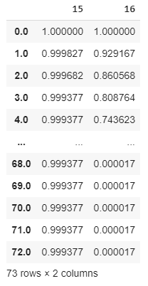
The customer in column 15 is expected to be 99.9% alive after 73 months from now, while that in 16 is expected to have a 74.4% probability of alive after only 4 months.

从现在起73个月后，第15列中的客户预计还可以存活99.9％，而在第16列中的客户仅需要4个月就可以存活74.4％。

Calculate Expected Loss

计算预期损失

We can use these survival probabilities to identify the specific month for each customer where his/her likelihood of survival falls below a certain threshold. Depending on the use case, we can choose any percentile, but for our project, we’ll use the median through the median_survival_times method. qth_survival_times can be used for any other percentile.

我们可以使用这些生存概率为每个客户确定其生存可能性低于特定阈值的特定月份。 根据使用情况，我们可以选择任何百分位数，但是对于我们的项目，我们将通过中位数median_survival_times方法使用中位数。 qth_survival_times可以用于任何其他百分比。

The output of the median_survival_times method is a single row representing the future month where the survival probability of each censored/alive customer falls below the median survival probability:

median_survival_times方法的输出是一行，代表未来月份，其中每个被审查/处于活动状态的客户的生存率都低于中值生存率：

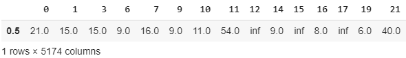
inf basically means that this customer is almost sure to be alive.

inf基本上意味着该客户几乎肯定还活着。

Next up, we will perform the following:

接下来，我们将执行以下操作：

• Concatenate the transposed output of median_survival_times with CustomerID and respective MonthlyCharges (that we set aside at the very beginning). This will allow us to tie back our predictions to each specific customer and their monthly charges

  将中median_survival_times的转置输出与CustomerID和相应的MonthlyCharges(我们一开始就搁置)连接在一起。 这将使我们能够将我们的预测与每个特定客户及其月度费用相关联

• Calculate each customer’s expected loss if they were to churn today by multiplying their monthly charges with their expected churn month
  通过将每个月的费用乘以他们的预期流失月份来计算每个客户今天流失的预期损失

• For customers with inf as their expected churn month, replace inf with a heuristic, maybe 24, corresponding to a 2-year contract. This would allow us to estimate these customer’s associated expected loss if they were to leave us today on the assumption that they will stay with us for at least 24 months

  对于inf为预期客户流失月份的客户，请用启发式(可能为24)替换inf ，对应于2年的合同。 如果他们今天离开我们，假设他们将与我们在一起至少24个月，这将使我们能够估计这些客户的相关预期损失

Our data, sorted on descending order of expected loss, looks something like this now:

我们的数据按预期损失的降序排列，现在看起来像这样：

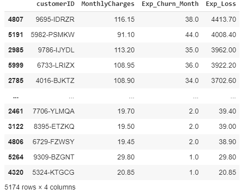
We have now identified the customers who pose the highest monetary risk to us if they were to leave us today.

现在，我们已经确定了如果今天离开我们对我们构成最大货币风险的客户。

Calculate Estimated Revenue Uplift

计算预计的收入提升

What can we do to retain them? The coefficients from our CPH model and associated KM survival curves indicate what features we need to focus on to retain our current customers. However, let’s now try to estimate the monetary benefit if we can convince our customers to sign up for these specific features that prevent churn if they are not already subscribed to them.

我们如何保留他们？ CPH模型的系数和相关的KM生存曲线表明了我们需要关注哪些功能来留住当前客户。 但是，现在，如果我们可以说服我们的客户注册这些特定功能(如果尚未订阅的话，则可以防止流失)，那么我们就尝试估算其货币收益。

Accordingly, we will estimate the potential uplift in our revenue for the following features if we can get a customer who does not have the following to subscribe/sign on for them.

因此，如果我们可以让没有以下内容的客户订阅/登录，我们将估计以下功能的潜在收入增长。

• a 1-year contract
  一年合约
• a 2-year contract
  两年合约
• DSL
  DSL
• automatic payment through bank transfer
  通过银行转帐自动付款
• automatic payment through credit card
  通过信用卡自动付款

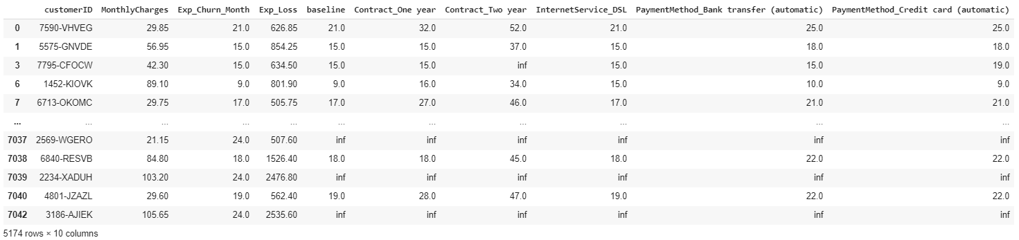
We will now calculate the potential uplift for each of the above covariates and each customer through nested for loops under hypothetical scenarios. For example, we can calculate the revised expected churn month if he signs up for a one year contract in case he was not on a one year contract.

现在，我们将通过假设场景下的嵌套for循环，为上述每个协变量和每个客户计算潜在的提升。 例如，如果他签了一年合同(如果他没有一年合同)，我们可以计算出修订后的预期客户流失月份。

Our initial uplift analysis results in something like this:

我们的初步隆起分析结果如下：

Now we have the revised expected churn month for each customer if we can sign up for a specific feature, ceteris paribus. For example, we can expect customer 7590-VHVEG to stay with us for 11 more months if we can just get him to sign up for a one year contract, ceteris paribus. Or he is expected to stay for 4 additional months if he sets up automatic payments, ceteris paribus.

现在，如果我们可以注册特定功能( ceteris paribus) ，我们将为每个客户修订预期的客户流失月份。 例如，我们可以预期客户7590-VHVEG和我们呆在一起提供11个月，如果我们可以只让他签署了一年的合同， 其他条件不变 。 或者，如果他设置自动付款，则他将再停留4个月， ceteris paribus 。

As noted earlier, we have some very good customers with low churn risk, represented by inf values in the baseline month. We do not need to focus our marketing efforts on them for the time being. So we will exclude them from further analysis.

如前所述，我们有一些非常好的客户，客户流失风险低，以基准月份的inf值表示。 我们暂时不需要将营销精力集中在它们上。 因此，我们将其排除在进一步分析之外。

Let us go a step further and see the customer-wise financial impact of each potential upgrade over the expected revised lifetime, instead of just the expected additional months. This is a simple calculation whereby we take the difference between the baseline and revised churn month for each covariate and multiply that by the monthly charges.

让我们更进一步，看看在预期修订的生命周期内，而不只是预期的额外月份，每次潜在升级对客户的财务影响 。 这是一个简单的计算，由此我们将每个协变量的基准流失月份和修订流失月份之间的差异乘以月度费用。

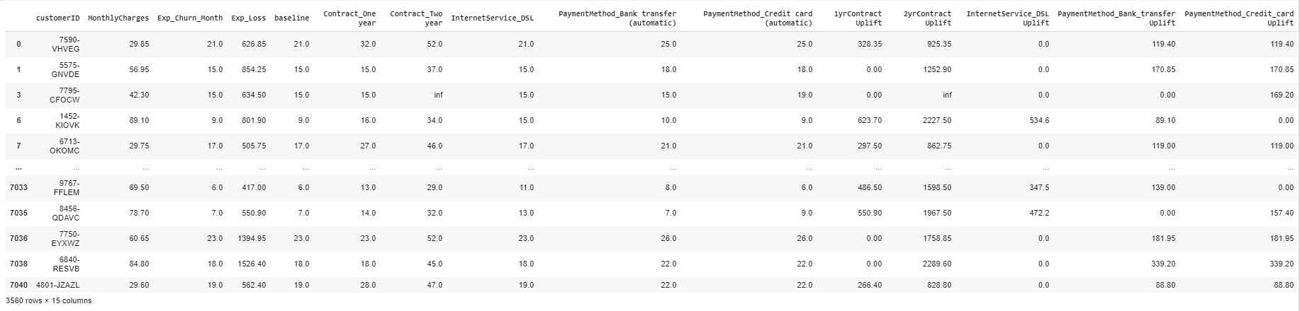
So now we know the following for customer 7590-VHVEG:

因此，现在我们为客户7590-VHVEG了解以下内容：

• additional revenue of $328.35 over his expected increased lifetime if he signs up to a one year contract, ceteris paribus

  在他签署长达一年的合同预计他的寿命增加的$ 328.35的额外收入， 其他条件不变

• additional revenue of $925.35 over his expected increased lifetime if he signs up to a 2-year contract, ceteris paribus

  在他签署长达2年的合同，他的预期寿命增加的$ 925.35的额外收入， 其他条件不变

• additional revenue of $119.4 over his expected increased lifetime if he converts to one of the automatic payment methods, ceteris paribus

  如果他转换为自动付款方式之一， ceteris paribus ，则可以在预期的有效期内增加119.4美元的收入

All the code related to churn prediction and prevention analysis is below:

与客户流失预测和预防分析有关的所有代码如下：

# function for creating KM curves segmented by categorical variables
def plot_categorical_KM_Curve(feature, t='tenure', event='Churn', df=data_kmf, ax=None):
    for cat in df[feature].unique():
        idx = df[feature] == cat
        kmf.fit(df[idx][t], event_observed=df[idx][event], label=cat)
        kmf.plot(ax=ax, label=cat)
# call the above function and plot 4 KM Curves
fig, ((ax1, ax2), (ax3, ax4)) = plt.subplots(nrows = 2, ncols = 2, figsize=(20,10))
# PaymentMethod
plot_categorical_KM_Curve(feature='PaymentMethod', ax=ax1)
ax1.set_title('Kaplan-Meier Survival Curve by Payment Method')
ax1.set_xlabel('Customer Tenure (Months)')
ax1.set_ylabel('Customer Survival Chance (%)')
# Contract
plot_categorical_KM_Curve(feature='Contract', ax=ax2)
ax2.set_title('Kaplan-Meier Survival Curve by Contract Duration')
ax2.set_xlabel('Customer Tenure (Months)')
ax2.set_ylabel('Customer Survival Chance (%)')
# InternetService
plot_categorical_KM_Curve(feature='InternetService', ax=ax3)
ax3.set_title('Kaplan-Meier Survival Curve by Internet Service')
ax3.set_xlabel('Customer Tenure (Months)')
ax3.set_ylabel('Customer Survival Chance (%)')
# PhoneService
plot_categorical_KM_Curve(feature='PhoneService', ax=ax4)
ax4.set_title('Kaplan-Meier Survival Curve by Phone Service')
ax4.set_xlabel('Customer Tenure (Months)')
ax4.set_ylabel('Customer Survival Chance (%)');


# Filter censored customers
censored_data = data[data['Churn'] == 0]
# Carve out the tenure column for each customer
censored_data_last_obs = censored_data['tenure']
# Predict the survival function for each customer from this day onwards
conditioned_sf = cph.predict_survival_function(censored_data, conditional_after = censored_data_last_obs)


# Predict the month where the survival probability falls below the median
predictions_50 = lifelines.utils.median_survival_times(conditioned_sf)


# concatenate the expected churn month with customerID and MonthlyCharges to allow customer-specific analysis
customer_predictions = pd.concat([customerID[['customerID', 'MonthlyCharges']], predictions_50.T], axis = 1)
# Rename the column returned by median_survival_times function
customer_predictions.rename(columns = {0.5: 'Exp_Churn_Month'}, inplace = True)
# Add another column for the expected loss if these customers were to leave us today
customer_predictions['Exp_Loss'] = customer_predictions['MonthlyCharges'] * customer_predictions['Exp_Churn_Month']


# Assign 24 to inf values in Exp_Churn_Month
customer_predictions['Exp_Churn_Month'].replace([np.inf, -np.inf], 24, inplace = True)
# Recalculate the customer_predictions table and sort it
customer_predictions['Exp_Loss'] = customer_predictions['MonthlyCharges'] * customer_predictions['Exp_Churn_Month']
customer_predictions.sort_values(by = ['Exp_Loss'], ascending = False)


# UPLIFT ANALYSIS
# Store the column names to be analysed in a list
upgrades = ['Contract_One year', 'Contract_Two year', 'InternetService_DSL', 
	    'PaymentMethod_Bank transfer (automatic)', 'PaymentMethod_Credit card (automatic)']
# Define an empty dictionary to hold the results
results_dict = {}
# For each of the potential upgrades, loop through each individual customer to determine the increase in expected median churn month
for customer in customer_predictions.index:  
    # save the actual cutomer data as a series
    actual = censored_data.loc[[customer]]
    # same as actual but this series will be used to evaluate hypothetical scenarios
    change = censored_data.loc[[customer]] 
    # calculate the base median churn month
    results_dict[customer] = [cph.predict_median(actual, conditional_after = 
						 censored_data_last_obs[customer])]
    for upgrade in upgrades:
        # hypothetical scenario where customer signs up for this particular upgrade
	change[upgrade] = 1 if list(change[upgrade]) == 0 else 1
        # calculate the revised median churn month under the above hypothetical scenario
	results_dict[customer].append(cph.predict_median(change, conditional_after = 
								 censored_data_last_obs[customer]))
        # bring the change series back to the original state (i.e. undo the effect of the hypothetical scenario)
	change = censored_data.loc[[customer]]
# Convert dictionary to a DF and transpose the resultant DF back to the required format (each customer in a separate row)
results_df = pd.DataFrame(results_dict).T 
# add 'baseline' to the beginning of upgrades list. This new list will be used to rename the columns of results_df
column_names = upgrades
column_names.insert(0, 'baseline')
results_df.columns = column_names
# Concat this new df with customer_predictions DF
upgrade_analysis = pd.concat([customer_predictions, results_df], axis = 1) 


# replace inf values in baseline column with NaN before dropping these rows
upgrade_analysis['baseline'].replace([np.inf, -np.inf], np.nan, inplace = True)
upgrade_analysis.dropna(subset = ['baseline'], axis=0, inplace = True)


# Calculate the difference in months between baseline and each feature's revised tenures and multiple this difference by MonthlyCharges
upgrade_analysis['1yrContract Uplift'] = (upgrade_analysis['Contract_One year'] -
					  upgrade_analysis['baseline']
					 ) * upgrade_analysis['MonthlyCharges'] 
upgrade_analysis['2yrContract Uplift'] = (upgrade_analysis['Contract_Two year'] -
					  upgrade_analysis['baseline']
					 ) * upgrade_analysis['MonthlyCharges']
upgrade_analysis['InternetService_DSL Uplift'] = (upgrade_analysis['InternetService_DSL'] -
						  upgrade_analysis['baseline']
						 ) * upgrade_analysis['MonthlyCharges'] 
upgrade_analysis['PaymentMethod_Bank_transfer Uplift'] = (
	upgrade_analysis['PaymentMethod_Bank transfer (automatic)'] - 
	upgrade_analysis['baseline']) * upgrade_analysis['MonthlyCharges'] 
upgrade_analysis['PaymentMethod_Credit_card Uplift'] = (
	upgrade_analysis['PaymentMethod_Credit card (automatic)'] -
	upgrade_analysis['baseline']) * upgrade_analysis['MonthlyCharges']

结论 (Conclusion)

Now we have some actionable insights into not only which of our customers are at risk of churning, but some actionable insights as well with regards to expected time to churn and potential uplift in revenue through the introduction of customer-specific strategies.

现在，我们不仅对哪些客户有搅局的风险有切实可行的见解，而且对于通过引入特定于客户的战略而预期的流失时间和潜在的收入增长方面也有一些可行的见解。

The complete Jupyter notebook is available on GitHub here.

完整的Jupyter笔记本可在GitHub上找到 。

As always, feel free to reach out to me if you would like to discuss anything related to data analytics, machine learning, financial and credit risk analysis.

与往常一样，如果您想讨论与数据分析，机器学习，财务和信用风险分析有关的任何事情，请随时与我联系 。

Till next time, code on!

直到下一次，编码！

翻译自: https://towardsdatascience.com/how-to-not-predict-and-prevent-customer-churn-1097c0a1ef3b

客户流失预测