保险理赔 kaggle_R上的Kaggle大篷车保险挑战的功能选择

保险理赔 kaggle

Recapping from the previous post, this post will explains the feature selection to the Kaggle caravan insurance challenge before we feed the features into machine learning algorithms (probably the next post), which aims to identify those customers who are most likely to purchase caravan policies based on 85 historic socio-demographic and product-ownership data attributes.

在前一篇博文的基础上，本博文将向我们介绍机器学习算法(可能是下一篇博文)之前，向Kaggle大篷车保险挑战挑战介绍功能选择，目的是确定最有可能购买大篷车保单的客户基于85个历史社会人口统计数据和产品所有权数据属性。

名义数据属性 (Nominal data attributes)

Out of the 85 historic data attributes, they consist of nominal and ordinal attributes. Nominal attributes are data in the forms of names but there’s no clear order between them. Some examples are Male vs Female, Blood type O vs Blood Type A vs Blood Type B or even zipcode. Ordinal attributes are data with a clear distinct orders between each level of the data attribute like cholesterol level low vs medium vs high or happiness level on a scale of 1 to 10. As a result, we have to convert the nominal attributes to factor form before we can begin feeding our training data into any ML algorithms.

在85个历史数据属性中，它们由名义和有序属性组成。 名义属性是名称形式的数据，但是它们之间没有明确的顺序。 例如，男性对女性，O型血对A型血对B型血，甚至是邮政编码。 序数属性是数据属性的每个级别之间的清晰明显的顺序，例如胆固醇水平从低到中，从高到高或从1到10的幸福水平。结果，我们必须先将名义属性转换为因子形式我们可以开始将训练数据输入任何ML算法中。

This can be easily done in R using library packagedplyr and the command factor.

使用库包dplyr可以在R中轻松完成此操作 和命令因素。

功能选择 (Feature selection)

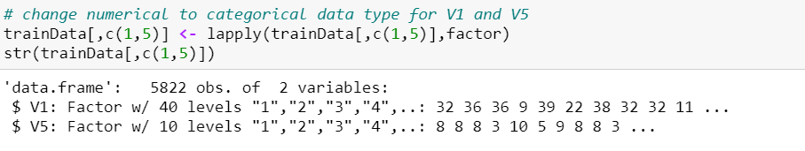
After converting both V1 and V5 attributes into factor format, note that the initial 85 data attributes have been increased to 133 as V1 consists of 40 different categories while V5 has 10. Feeding 133 attributes into any ML algorithms is not feasible, which is why we have to perform feature selection to train our model faster.

将V1和V5属性都转换为因子格式后，请注意，最初的85个数据属性已增加到133，因为V1由40个不同类别组成，而V5具有10个类别。将133个属性输入任何ML算法都不可行，这就是为什么我们必须执行特征选择以更快地训练我们的模型。

Subset selection, stepwise selection and Lasso regularisation are some of the methods available to identify those predictor variables that are significantly better to predict the target variable, and they are especially useful if the number of predictor variables available is large which in particularly, useful in this assignment as we have a total of 133 predictor variables available to us.

子集选择，逐步选择和套索正则化是可用来识别那些更好地预测目标变量的预测变量的一些方法，如果可用的预测变量的数量很大，则它们特别有用，在此方面特别有用分配，因为我们总共可以使用133个预测变量。

Firstly for subset selection, as the number of predictor variables available here is large (i.e. 133), we will have to train 2¹³³ models which is computationally expensive in terms of time complexity. Hence, we will not consider the method of exhaustive subset selection.

首先，对于子集选择，由于此处可用的预测变量数量很多(即133)，我们将不得不训练2 13 3模型，这在时间复杂度方面在计算上是昂贵的。 因此，我们将不考虑穷举子集选择的方法。

向前逐步选择 (Forward stepwise selection)

The next method we consider is stepwise collection, which includes forward stepwise selection and backward stepwise selection. We can use the regsubsets function from leaps package to do them. Forward stepwise selection is a type of stepwise regression which begins with an empty model and adds in data features one by one, with the one that improves the model the most (i.e. the most significant one).

我们考虑的下一个方法是逐步收集，包括向前逐步选择和向后逐步选择。 我们可以使用regsubsets功能从leaps包来完成它们。 正向逐步选择是一种逐步回归的类型，它从一个空模型开始，并逐一添加数据特征，其中一个特征对模型的改进最大(即，最显着)。

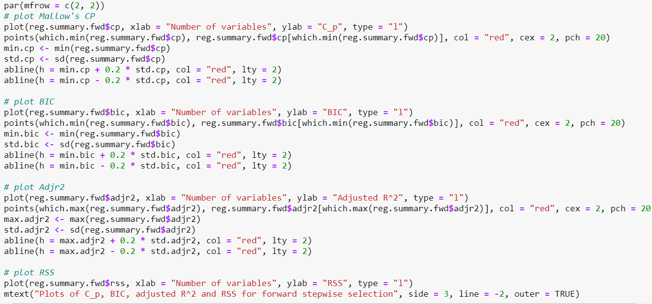
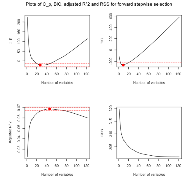
The summary of the output is not easy to read, which is why we can use some other measurements or plots to visualise our results from forward stepwise selection more easily. We consider the following 3 measures:

输出的摘要不容易阅读，这就是为什么我们可以使用其他一些测量值或图表来更直观地显示正向逐步选择结果的原因。 我们考虑以下3种措施：

1) Mallow’s CP 2) Bayesian Information Criterion 3) Adjusted 𝑅²

1) Mallow的CP 2)贝叶斯信息准则3)调整后的²

These measures will add penalty to the residual sum of squares for the number of variables (i.e. complexity) in the model. Since the more number of predictor variables we fit into our model, the complexity increases and the residual sum of squares of the model will be expected to decrease. Our goal is to find a model that has a low residual sum of squares but we will not want to fit a model with all the variables available because it would result in overfitting since as shown in our plot, RSS is lowest with 85 predictor variables in our model. Hence based on the above 3 measures, we will want to find a small value for Mallow’s CP and Bayesian Information Criterion, and a large value for adjusted 𝑅².

这些措施将增加模型中变量数量(即复杂性)的残差平方和的惩罚。 由于我们将更多的预测变量放入模型中，因此复杂度增加，并且模型的残差平方和将减少。 我们的目标是找到一个残差平方和低的模型，但我们不希望使用所有可用变量来拟合该模型，因为这会导致过度拟合，因为如图所示，RSS最低，其中85个预测变量我们的模型。 因此，基于以上三个度量，我们将希望为Mallow的CP和贝叶斯信息准则找到一个较小的值，为经过调整的²²找到一个较大的值。

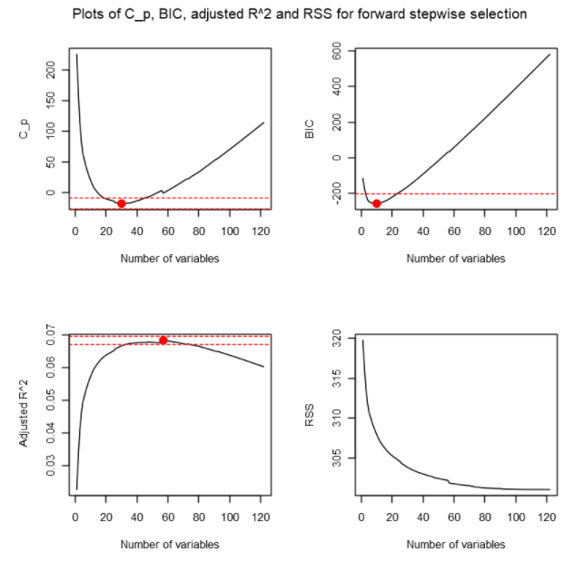
Based on the plots, according to Mallow’s CP, the best performer is the model with 30 predictor variables. According to BIC, the best performer is the model with 10 predictor variables. According to Adjusted 𝑅², the best model is the model with 57 predictor variables. If we were to look at the number of variables that are within 0.2 standard deviations from the optimal, we can see that 25 number of predictor variables seem to satisfy the 3 criteria.

根据这些图，根据Mallow的CP，表现最好的模型是具有30个预测变量的模型。 根据BIC，表现最好的是具有10个预测变量的模型。 根据Adjusted𝑅²，最佳模型是具有57个预测变量的模型。 如果我们查看与最佳值相差0.2个标准差的变量数量，则可以看到25个预测变量似乎满足了3个标准。

We can also conclude here that a model with 9 or less predictor variables is considered underfitting and model with 58 predictor variables or more is considered overfitting.

我们还可以在这里得出结论，将具有9个或更少预测变量的模型视为拟合不足，而将具有58个或更多预测变量的模型视为拟合过度。

We get the top 25 recommended variables by forward stepwise selection.

通过向前逐步选择，我们获得了前25个推荐变量。

向后逐步选择 (Backward stepwise selection)

We do the same for backward stepwise selection as what we did in forward stepwise selection. The only difference is that this method will first use all available features, then remove one by one those that’s not significant. We can just define the method = ‘backward’ to apply backward stepwise selection.

对于后向逐步选择，我们进行的操作与在向前逐步选择中所做的相同。 唯一的区别是此方法将首先使用所有可用功能，然后将不重要的功能一一删除。 我们可以定义方法='backward'来应用后退逐步选择。

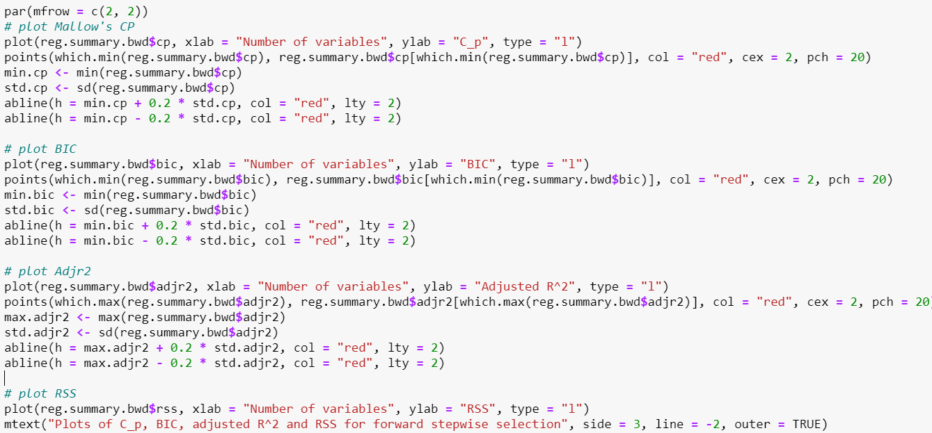
Similar to Forward Stepwise Selection, we observe the plots for Mallow’s CP, BIC and Adjusted 𝑅².

类似于正向逐步选择，我们观察了Mallow的CP，BIC和调整后的²²的图。

Based on the plots, according to Mallow’s CP, the best performer is the model with 27 predictor variables. According to BIC, the best performer is the model with 9 predictor variables. According to Adjusted 𝑅², the best model is the model with 46 predictor variables.

根据这些图，根据Mallow的CP，表现最好的模型是具有27个预测变量的模型。 根据BIC，表现最好的是具有9个预测变量的模型。 根据调整后的𝑅²，最好的模型是具有46个预测变量的模型。

If we were to look at the number of variables that are within 0.2 standard deviations from the optimal, we can see that 21 number of predictor variables seem to satisfy the 3 criteria. We can also conclude in this Backward Stepwise Selection that that a model with 8 or less predictor variables is considered underfitting and model with 47 predictor variables or more is considered overfitting.

如果我们查看与最佳值相差0.2个标准差的变量数量，则可以看到21个预测变量似乎满足了3个标准。 我们还可以在此“逐步逐步选择”中得出结论，将具有8个或更少预测变量的模型视为拟合不足，而将具有47个或更多预测变量的模型视为拟合过度。

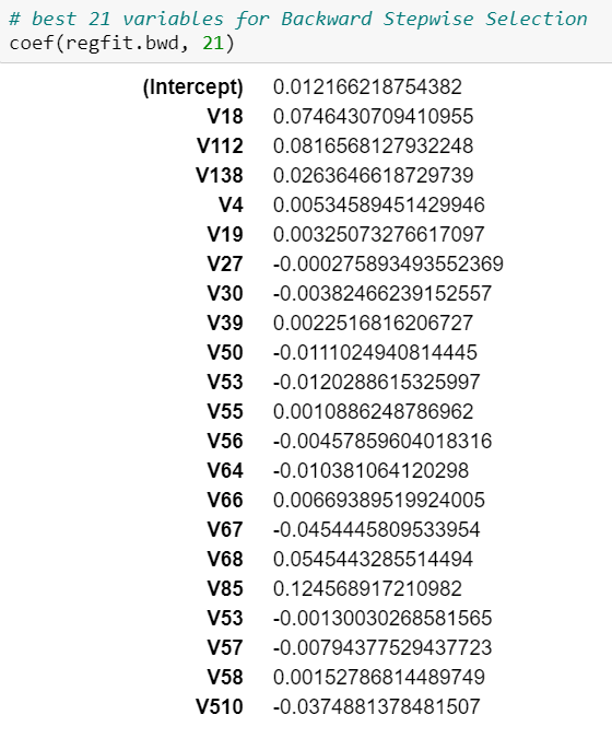
Let’s get the 21 predictor variables recommended by Backward Stepwise Selection.

让我们获取“向后逐步选择”推荐的21个预测变量。

Variables that appeared in both methods:1) V1.8 — Cust Subtype — Middle class families2) V1.12 — Cust Subtype — Affluent young families3) V1.38 — Cust Subtype — Traditional families4) V4 — Avg age5) V5.7 — Cust Maintype — Retired and Religeous6) V5.8 — Cust Maintype — Family with grown ups7) V5.10 — Cust Maintype — Farmers8) V19 — High status9) V27 — Social class B210) V50 — Contribution lorry policies11) V53 — Contribution agricultural machines policies12) V56 — Contribution private accident insurance policies13) V66 — Number of third party insurance (firms)14) V67 — Number of third party insurane (agriculture)15) V68 — Number of car policies

两种方法中都出现的变量：1)V1.8-房客亚型-中产阶级家庭2)V1.12-房客亚型-富裕的年轻家庭3)V1.38-房客亚型-传统家庭4)V4-平均年龄5)V5.7-客户的主要类型-退休和宗教6)V5.8-客户的主要类型-长大的家庭7)V5.10-客户的主要类型-农民8)V19-较高的身份9)V27-社会等级B210)V50-劳务费政策11)V53-劳务农机保单12)V56-私人事故保险13，V66-第三方保险(公司)数量14)V67-第三方保险(农业)数量15)V68-汽车保单数量

Variables that appeared in only Forward Stepwise Selection:1) V1.10 — Cust Subtype — Stable family2) V5.4 — Cust Maintype — Career Loners3) V5.5 — Cust Maintype — Living well4) V14 — Household without children5) V16 — High level education6) V25 — Social class Ae7) V37 — Income < 30.0008) V51 — Contribution trailer policies9) V52 — Contribution tractor policies10) V76 — Number of life insurances

仅在正向逐步选择中出现的变量：1)V1.10 —住户子类型—稳定的家庭2)V5.4 —住户主类型—职业成才3)V5.5 —住户主类型—生活得很好4)V14 —没有孩子的家庭5)V16 —高等级教育6)V25-社会等级Ae7)V37-收入<30.0008)V51-供款拖车保单9)V52-供款拖拉机保单10)V76-人寿保险数量

Variables that appeared in only Backward Stepwise Selection:1) V5.3 — Cust Maintype — Average Family2) V30 — Rented house3) V39 — Income 45–75.0004) V55 — Contribution life insurances5) V64 — Contribution social security insurance policies6) V85 — Number of social security insurance policies

仅出现在向后逐步选择中的变量：1)V5.3 —客户的主要类型—平均家庭2)V30-租住的房屋3)V39-收入45-75.0004)V55-缴费型人寿保险5)V64-缴费型社会保障保险6)V85-编号社会保障保险单

Note that we use the notation V1.x and V5.y where x and y represents the category in V1 and V5 respectively.

请注意，我们使用符号V1.x和V5.y ，其中x和y分别表示V1和V5中的类别。

套索正则化 (Lasso Regularisation)

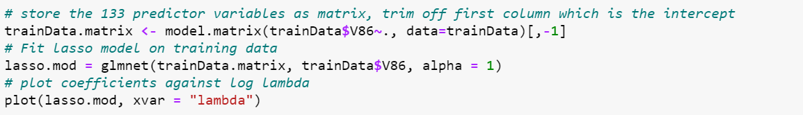
Next, we consider Lasso Regularisation which is one approach available to perform feature selection automatically. The Lasso Regulariation will introduce a shrinkage perimeter which will shrink the coefficient estimates towards zero. For those variables with coefficient estimates equal to zero, we can conclude that these variables are not related to the target variable which is why we can use Lasso Regularisation for feature selection. We use the glmnet function from glmnet package to help us build a Lasso model. Note that setting alpha=1 means we are considering lasso, if we were to consider ridge regression, alpha=0.

接下来，我们考虑套索正则化，这是一种可以自动执行特征选择的方法。 套索正则化将引入收缩周长，该收缩周长会将系数估计值收缩为零。 对于那些系数估计等于零的变量，我们可以得出结论，这些变量与目标变量无关，这就是为什么我们可以使用套索正则化进行特征选择的原因。 我们使用glmnet包中的glmnet函数来帮助我们建立套索模型。 请注意，设置alpha = 1表示我们正在考虑套索，如果要考虑岭回归，则alpha = 0。

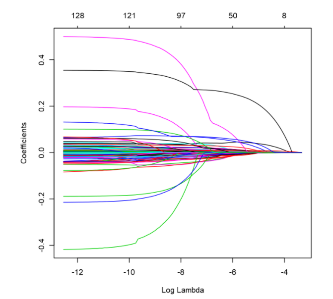
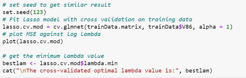
We see from the plot that as the shrinkage perimeter (i.e.lambda) increases, the coefficients will gradually approach zero. The issue now will be what should be the value of lambda that we take to decide the ideal number of predictor variables. We can consider the approach of cross validation to select the optimal value of lambda using cv.glmnet . Note that we set.seed(123) to be able to reproduce any results for checking purposes.

从图中可以看出，随着收缩周长(ielambda)的增加，系数将逐渐接近零。 现在的问题将是我们决定理想的预测变量数量时应采用的lambda值是多少。 我们可以考虑使用cv.glmnet交叉验证方法来选择lambda的最佳值。 请注意，我们将set.seed(123)设置为能够复制任何结果以进行检查。

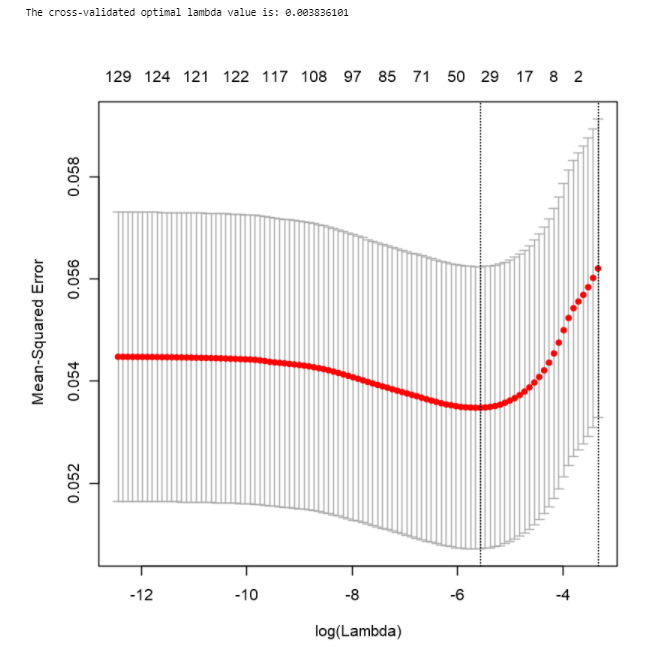
After running cross-validation, we get the most optimal lambda value to be 0.003836101 in which we can use this lambda value and retrain our Lasso model and identify those predictor variables that have estimated coefficients to be 0.

经过交叉验证后，我们得到的最佳lambda值为0.003836101，在其中我们可以使用该lambda值并重新训练我们的Lasso模型，并识别那些估计系数为0的预测变量。

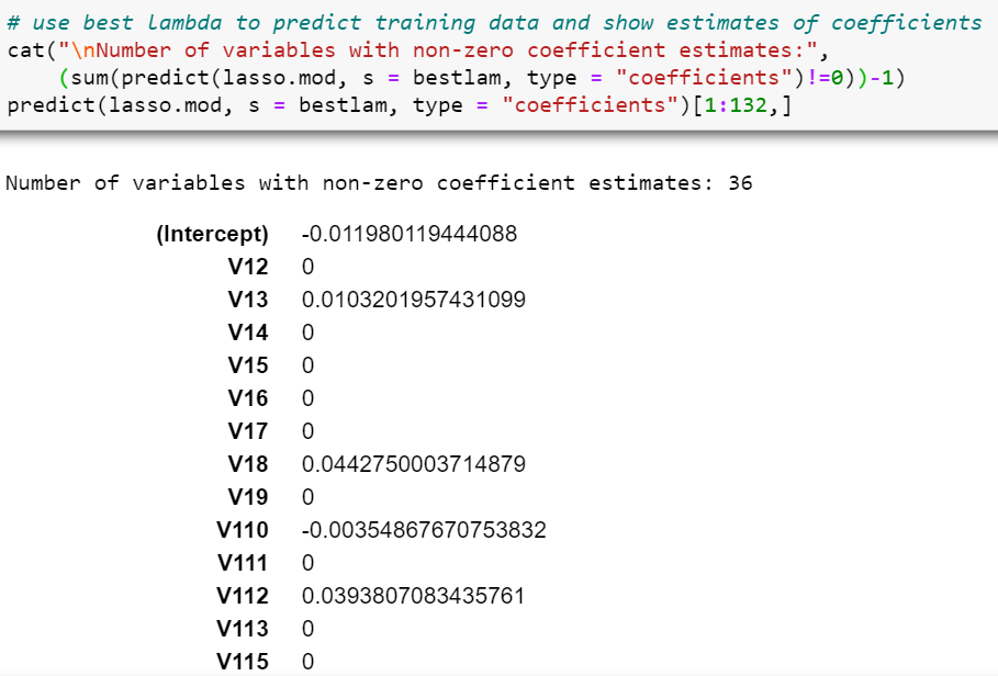
With this optimal lambda value, the number of predictor variables with non-zero coefficient estimates is 36 (37–1 intercept), and these variables are:

使用此最佳lambda值，具有非零系数估计的预测变量的数量为36 (37-1截距)，这些变量是：

1) V1.3 — High status seniors2) V1.8 — Middle class families3) V1.10 — Stable family4) V1.12 — Affluent young families5) V1.23 — Young and rising6) V1.38 — Traditional families7) V4 — Avg age8) V5.2 — Driven Growers9) V5.4 — Career Loners10) V5.5 — Living well11) V5.10 — Farmers12) V7 — Protestant13) V9 — No religion14) V10 — Married15) V11 — Living together16) V16 — High level educationn17) V18 — Lower level education18) V21 — Farmer19) V30 — Rented house20) V32–1 car21) V40 — Income 75–122.00022) V41 — Income >123.00023) V42 — Average income24) V43 — Purchasing power class25) V44 — Contribution private third party insurance26) V46 — Contribution third party insurane (agriculture)27) V47 — Contribution car policies28) V57 — Contribution family accidents insurance policies29) V58 — Contribution disability insurance policies30) V59 — Contribution fire policies31) V68 — Number of car policies32) V73 — Number of tractor policies33) V81 — Number of surfboard policies34) V82 — Number of boat policies35) V83 — Number of bicycle policies36) V85 — Number of social security insurance policies

1)V1.3-高级别老年人2)V1.8-中产阶级家庭3)V1.10-稳定的家庭4)V1.12-富裕的年轻家庭5)V1.23-年轻且正在崛起6)V1.38-传统家庭7)V4-平均年龄8)V5.2 —有驱动力的种植者9)V5.4 —职业导向者10)V5.5 —生活良好11)V5.10 —农民12)V7 —新教徒13)V9 —不信宗教14)V10 —已婚15)V11 —同居16)V16 —高学历n17)V18-低学历18)V21-农民19)V30-租住的房屋20)V32-1汽车21)V40-收入75-122.00022)V41-收入> 123.00023)V42-平均收入24)V43-购买力等级25)V44-私人私人第三方保险26)V46-第三方保险(农业)27)V47-私人汽车保单28)V57-意外家庭保险单29)V58-私人伤残保险单30)V59-私人火灾保单31)V68-汽车保单数量32 )V73-牵引车保单数量33)V81-冲浪板保单数量34)V82-Python数量t保单35)V83-自行车保单数量36)V85-社会保障保险单数量

概要(Summary)

Note that the following 6 variables appeared in all 3 feature selection method:1) V1.38 — Traditional families2) V1.12 — Affluent young families3) V1.38 — Traditional families4) V4 — Avg age5) V5.10 — Farmers6) V68 — Number of car policies

请注意，以下6个变量出现在所有3种特征选择方法中：1)V1.38-传统家庭2)V1.12-富裕的年轻家庭3)V1.38-传统家庭4)V4-平均年龄5)V5.10-农民6)V68 —汽车保单数量

We have identified 25 variables from forward stepwise selection, 21 from backward stepwise selection and 36 from lasso regression. They are definitely easier to feed into your ML algorithms compared to the initial 133 features. Hope these methods help in your data science projects with tons of data features identified initially!

我们从向前逐步选择中识别出25个变量，从反向逐步选择中识别出21个变量，从套索回归中识别出36个变量。 与最初的133个功能相比，它们绝对更易于输入到ML算法中。 希望这些方法能为您的数据科学项目提供帮助，帮助您初步确定大量的数据功能！

翻译自: https://medium.com/swlh/feature-selection-to-kaggle-caravan-insurance-challenge-on-r-bede801d3a66

保险理赔 kaggle