python可视化_python商业智能可视化

python可视化

Why are visualizations worth thousands of words? They have the power of telling stories and simplifying the interpretation of information. They help users detect patterns, insights and metrics, and as a result build better products and services. So they do really matter.

为什么可视化值得数千个单词？ 他们具有讲故事和简化信息解释的功能。 它们帮助用户检测模式，洞察力和指标，从而构建更好的产品和服务。 因此，它们确实很重要。

Visualizations are one of the most powerful tools in the set available to data analysts or data enthusiasts. In order to facilitate their creation, a wide range of softwares and languages has been developed. Maybe the usefulness of visualizations relates to the different interpretation that our brain naturally gives to images instead of large DataFrames, arrays or traditional tables allotted with data.

可视化是数据分析人员或数据爱好者可以使用的功能最强大的工具之一。 为了促进它们的创建，已经开发了各种各样的软件和语言。 可视化的有用性可能与我们的大脑自然对图像而不是分配有数据的大型DataFrame，数组或传统表的不同解释有关。

目录： (Table of contents:)

Importance of visualizations. (2 min read)

可视化的重要性。 (阅读2分钟)

Introduction to plot types with Python (8 min read)

使用Python绘制图形类型的简介(需读8分钟)

1.可视化的重要性 (1. Importance of Visualizations)

Tabulated data complicates conclusion extraction. Isolated numbers from their contexts, although structured in columns and rows accordingly to provide structure and orientate the user, are hard to make meaning out of. On the other hand, visualizations represent values at a glance. They show tabulated data in a simple way to easily and rapidly compare values, facilitating decision making.

列表数据使结论提取变得复杂。 从上下文中分离出来的数字，尽管相应地按行和列进行结构化，以提供结构和面向用户，但很难使含义变得清晰。 另一方面，可视化显示的值一目了然。 它们以简单的方式显示列表数据，以轻松，快速地比较值，从而有助于决策。

More important are these skills in Finance, Econometrics, Data Analytics and other math-related fields in which decision making is based on numeric fundamentals, usually hard to explain to not a savvy finance team member.

更重要的是金融，计量经济学，数据分析和其他数学相关领域的技能，在这些领域中，决策基于数字基础，通常很难解释为不是精通财务团队的成员。

Imagine yourself as an Asset Manager in an Investment Committee explaining your data-driven approach to asset allocation that creates an optimized portfolio with Machine Learning algorithms. Surely visualizations come in handy as argumentation for studies.

想象自己是投资委员会的资产经理，向您解释您的数据驱动资产配置方法，该方法通过机器学习算法创建了优化的投资组合。 可视化无疑可以派上用场作为研究的依据。

Big-data and huge-volume data processing have leveled-up the bar when it comes to storytelling-complexity of conclusions extracted from the analysis. In this context, user-friendly reports and other tailored presentations that can be recreated to specific audiences gain special value.

对于讲故事的复杂性(从分析中得出的结论)，大数据和海量数据处理已提高了门槛。 在这种情况下，可以为特定受众重新创建的用户友好型报告和其他量身定制的演示文稿具有特殊价值。

In this article I will not focus on specifically-designed tools to produce visualizations such as Tableau, Qlik and Power BI. Products within this category vary by capabilities and ease–of–use and are generally quick to set up, enabling users to access data from multiple sources. I will majorly focus in bringing you insights to more tailor-made visualizations with the application of our coding skills in Python, taking advantage of the Matplotlib a 2-D plotting library which has some neat tools to enable the creation of beautiful and flexible graphs and visualizations.

在本文中，我将不专注于专门设计的工具来产生可视化的表格，例如Tableau，Qlik和Power BI 。 此类别中的产品因功能和易用性而异，并且通常可以快速设置，从而使用户可以从多个来源访问数据。 我将主要专注于利用我们在Python中的编码技能，通过使用Matplotlib 2-D绘图库提供的见解，为更量身定制的可视化提供见解，该库具有一些简洁的工具，可用于创建漂亮而灵活的图形，以及可视化。

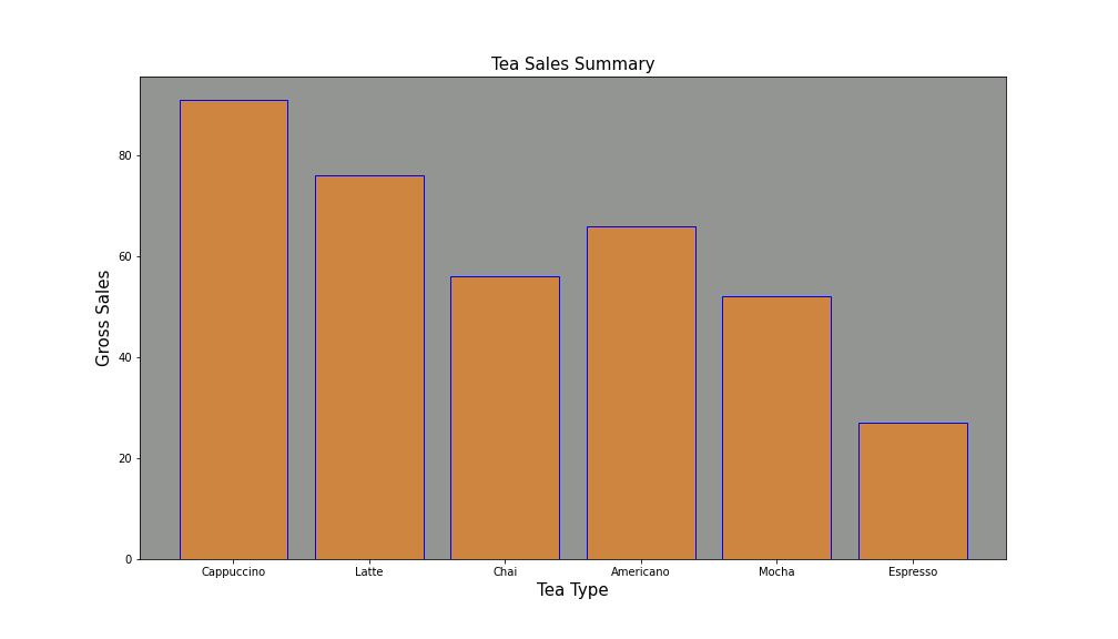
Let’s take a look on how data-interpretation is hugely improved with the use of data. Have a look at this DataFrame including different types of tea’s sales:

让我们看一下如何通过使用数据来极大地改善数据解释。 看一下这个DataFrame，其中包括不同类型的茶的销售：

In the following image you’ll see how it would be visually displayed with a Matplotlib bar-plot. Clearly, rapid conclusions can be made, such as best and worst selling tea-types, intermediate-selling ones and a comparisons between the magnitude of the sales of each tea type at a glance:

在下图中，您将看到如何用Matplotlib条形图直观地显示它。 显然，可以快速得出结论，例如最畅销和最畅销的茶类型，中等销售的茶类型以及每种茶的销售量之间的比较一目了然：

2.使用Python绘制图形类型简介 (2. Introduction to plot types with Python)

Installation process is pretty straight forward. Just open your terminal and insert the following command:

安装过程非常简单。 只需打开您的终端并插入以下命令：

 pip install matplotlib

A.线图 (A. Line Plot)

After having installed the library, we can jump on to plot creation. The first type we’re going to create is a simple Line Plot:

安装库之后，我们可以继续进行绘图创建。 我们要创建的第一种类型是简单的线图：

 # Begin by importing the necessary libraries:
import matplotlib.pyplot as plt

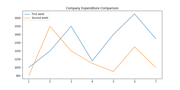
Suppose you want to plot your company’s one week expenditure compared to the previous week’s one the with the following input data:

假设您要使用以下输入数据来绘制公司一周的支出与上周的支出之比：

 # Days of the week:
days = [1, 2, 3, 4, 5, 6,7]
# Money spend one week 1
money_spent = [1000, 1200, 1500, 1080, 1400, 1650, 1350]
# Money spend one week 2
money_spent_2 = [900, 1500, 1200, 1050, 950, 1250, 1000] # Create figure:
fig = plt.figure(figsize=(10,5))
# Plot first week expenses:
plt.plot(days, money_spent)
# Plot second week expenses:
plt.plot(days, money_spent_2)
# Display the result:
plt.title('Company Expenditure Comparison')
plt.legend(['First week', 'Second week'])
plt.show()

Sample plot — Image by Author

样地—照片作者作者

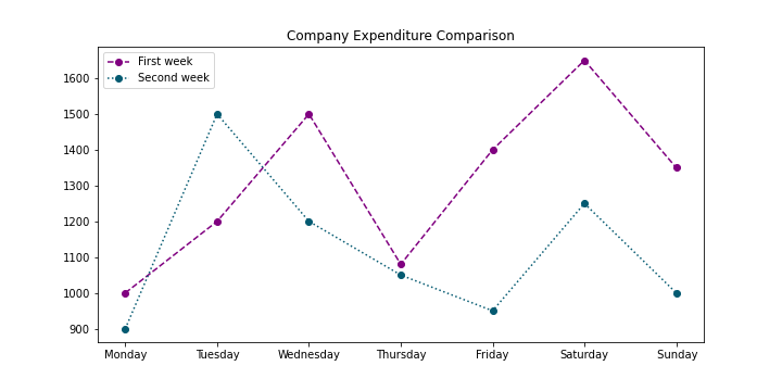
This plot can have some nice styling modifications with few lines of code:

该图可以用几行代码进行一些不错的样式修改：

 # Display the result:
ax = plt.subplot()
ax.set_xticks(range(1,8))
ax.set_xticklabels(['Monday', 'Tuesday', 'Wednesday', 'Thursday', 'Friday','Saturday',' Sunday'])
plt.title('Company Expenditure Comparison')
plt.legend(['First week', 'Second week'])
plt.show()

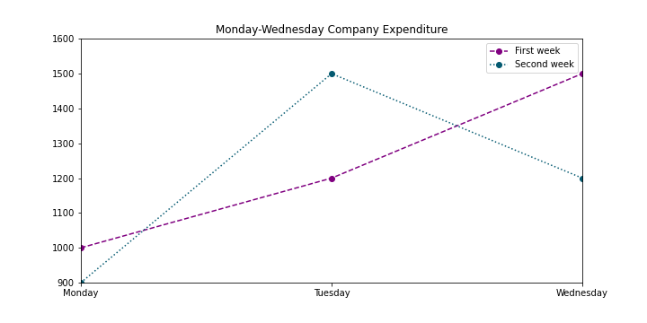
If you want to zoom-in to a particular spot you can do it with the plt.axis command with the input of the X and Y axis desired coordinates:

如果要放大到特定位置，可以使用plt.axis命令，并输入所需的X和Y轴坐标：

 plt.axis([1,3,900,1600])

子图 (Subplots)

Matplotlib library provides a way to plot multiple plots on a single figure. In order to create multiple plots inside one figure, configure the following arguments for the matplotlib.pyplot.subplots method as a generalization:

Matplotlib库提供了一种在单个图形上绘制多个图的方法。 为了在一个图形中创建多个图，请为matplotlib.pyplot.subplots方法配置以下参数作为概括：

 # Subplot creation
plt.subplots(nrows=1,ncols=1,sharex=False,sharey=False,squeeze=True,subplot_kw=None,gridspec_kw=None)

In case you don’t insert these parameters as they’re set by default, be sure to utilize the plt.subplot method to indicate the coordinates of the subplot to configure. Parameters:

如果您不插入默认设置的这些参数，请确保使用plt.subplot方法指示要配置的子图的坐标。 参数：

• nrows: Number of rows in the figure.

  nrows ：图中的行数。

• ncols: Number of columns in the figure.

  ncols ：图中的列数。

• plot_number: Index of the subplot inside the figure.

  plot_number ：图中内部子图的索引。

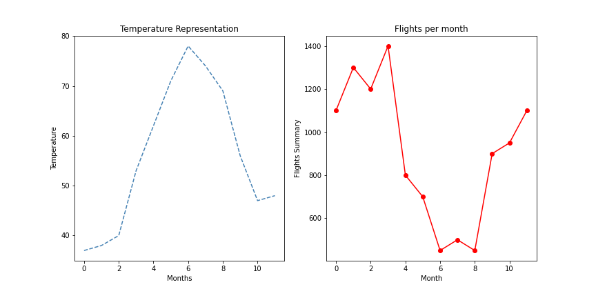
For e.g., suppose that you want to make a representation of temperature across the year in relation to flight sales during the same period with the following input data, just to find out if there’s any correlation between those variables:

例如，假设您要使用以下输入数据来表示同一时期内全年相对于航班销售的温度，只是要找出这些变量之间是否存在任何相关性：

 # Temperature and flight sales 
months = range(12)
temperature = [37, 38, 40, 53, 62, 71, 78, 74, 69, 56, 47, 48]
flights = [1100, 1300, 1200, 1400, 800, 700, 450, 500, 450, 900, 950, 1100] # Create figure:
fig = plt.figure(figsize=(12,6)) # Display the result - Plot 1:
plt.subplot(1,2,1)
# Plot temperatures:
plt.plot(months,temperature,color='steelblue',linestyle='--')
# Configure labels and title:
plt.xlabel('Months')
plt.ylabel('Temperature')
plt.title('Temperature Representation') # Display the result - Plot 2:
plt.subplot(1,2,2)
# Plot flights:
plt.plot(months,flights,color='red',marker='o')
plt.xlabel('Month')
# Configure labels and title:
plt.ylabel('Flights Summary')
plt.title('Flights per month')
plt.show()

Sample plot — Image by Author

样地—照片作者作者

B.并排条形图(B. Side-by-side Bar Chart)

I’ll skip visualizations of simple bar charts to focus on more business-related side-by-side charts. The basic command utilized for bar charts is plt.bar(x_values, y_values).

我将跳过简单条形图的可视化，将重点放在与业务相关的更多并排图表上。 条形图使用的基本命令是plt.bar(x_values，y_values)。

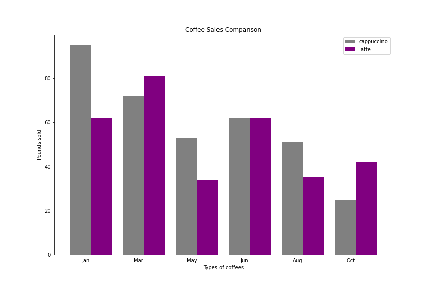
Side-by-side bar charts are used to compare two sets of data with the same types of axis values. Some examples of data that side-by-side bars could be useful for include:

并排条形图用于比较两组具有相同类型轴值的数据。 并排的条可能有用的一些数据示例包括：

• Population of more than one country over a period of time.
  一段时间内多个国家/地区的人口。
• Prices for different foods at more than one restaurant over a period of time.
  一段时间内，不止一家餐厅的不同食物的价格。
• Enrollments in different classes for male and female students.
  男女生不同班级的入学率。

We will use the following information to create the chart:

我们将使用以下信息来创建图表：

 # Values for X axis bar separation:
x_values1 = [0.8,2.8,4.8,6.8,8.8,10.8]
x_values2 = [1.6,3.6,5.6,7.6,9.6,11.6] # Sales by month and labels:
drinks = ["cappuccino", "latte", "chai", "americano", "mocha", "espresso"]
months_sales = ['Jan','Mar','May','Jun','Aug','Oct', 'Dec']
sales_cappuccino = [95, 72, 53, 62, 51, 25]
sales_latte = [62, 81, 34, 62, 35, 42]

Plot configuration looks something like this:

绘图配置如下所示：

 # Figure creation:
fig = plt.figure(figsize=(12,8)) # Subplot configuration:
ax = plt.subplot()
ax.set_xticks(range(1,12,2))
ax.set_xticklabels(months_sales) # Bar plot creation:
plt.bar(x_values1, sales_cappuccino, color='gray')
plt.bar(x_values2, sales_latte, color='purple') # Display plot:
plt.title("Coffee Sales Comparison")
plt.xlabel("Types of coffees")
plt.ylabel("Pounds sold")
plt.legend(labels=drinks, loc='upper right')
plt.show()

C.堆积条形图 (C. Stacked Bars Chart)

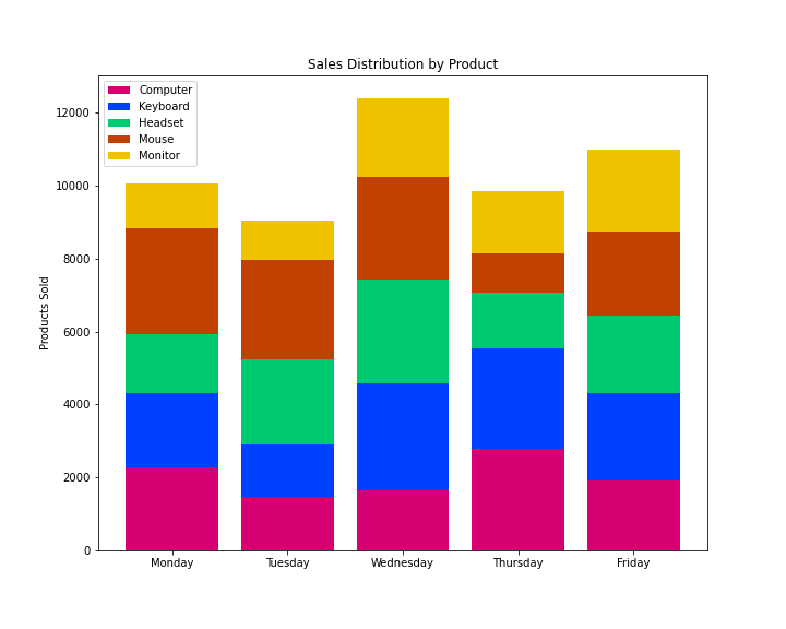
If we want to compare two sets of data while preserving knowledge of the total between them, we can also stack the bars instead of putting them side by side. We do this by using the keyword bottom.

如果我们要比较两组数据，同时又要保留它们之间的总数，则也可以堆叠这些条形，而不必将它们并排放置。 为此，我们使用关键字bottom 。

For e.g. suppose that we want to evaluate the distribution of our sales by product without losing perspective from total sales:

例如，假设我们要评估按产品划分的销售分布，而又不失总销售额的观点：

 # Product identification & Sales per product:
product = ['Computer', 'Keyboard', 'Headset', 'Mouse', 'Monitor']
sales_c = np.random.randint(1000,3000,5)
sales_k = np.random.randint(1000,3000,5)
sales_h = np.random.randint(1000,3000,5)
sales_m = np.random.randint(1000,3000,5)
sales_o = np.random.randint(1000,3000,5) # Configure bottoms to stack bars:
k_bottom = np.add(sales_c, sales_k)
h_bottom = np.add(k_bottom, sales_h)
m_bottom = np.add(h_bottom, sales_m) # Create figure and axes:
fig = plt.figure(figsize=(10,8))
ax = plt.subplot() # Plot bars individually:
plt.bar(range(len(sales_c)),sales_c, color='#D50071', label=product[0])
plt.bar(range(len(sales_k)),sales_k, bottom=sales_c, color='#0040FF',label=product[1])
plt.bar(range(len(sales_h)),sales_h, bottom=k_bottom, color='#00CA70',label=product[2])
plt.bar(range(len(sales_m)),sales_m, bottom=h_bottom, color='#C14200',label=product[3])
plt.bar(range(len(sales_o)),sales_o, bottom=m_bottom, color='#F0C300',label=product[4]) # Display graphs:
ax.set_xticks(range(5))
ax.set_xticklabels(['Monday','Tuesday', 'Wednesday', 'Thursday', 'Friday'])
plt.legend(loc='best')
plt.title('Sales Distribution by Product')
plt.ylabel("Products Sold")
plt.show()

D.饼图 (D. Pie Chart)

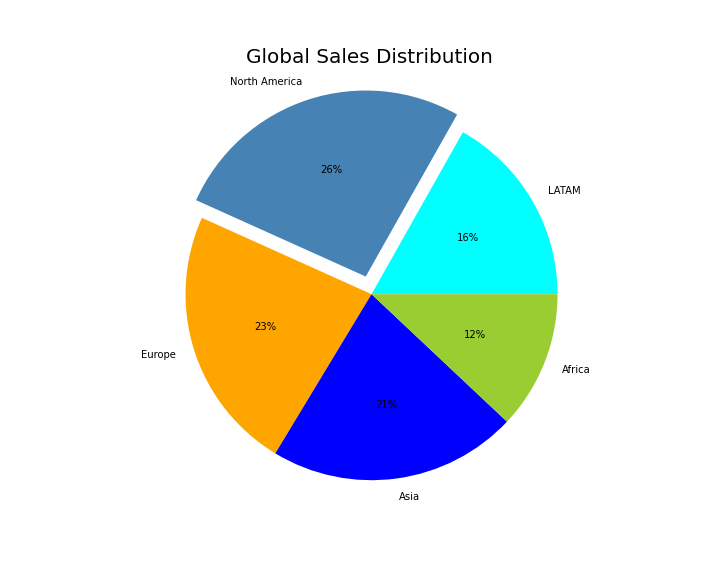
If we want to display elements of a data set as proportions of a whole, we can use a pie chart. In Matplotlib, you can make a pie chart with the command plt.pie, passing in the values you want to chart.

如果我们想将数据集的元素显示为整体的比例，则可以使用饼图。 在Matplotlib中，您可以使用命令plt.pie制作饼图，并传入要绘制的值。

We also want to be able to understand what each slice of the pie represents. To do this, we can either:

我们还希望能够理解馅饼的每个部分代表什么。 为此，我们可以：

• Use a legend to label each color.
  使用图例标记每种颜色。
• Put labels on the chart itself.
  在图表本身上放置标签。

One other useful labeling tool for pie charts is adding the percentage of the total that each slice occupies. Matplotlib can add this automatically with the keyword autopct. In addition, I’ll add the explode feature, which highlights selected pieces of the “pie”.

饼图的另一种有用的标签工具是将每个切片所占总数的百分比相加。 Matplotlib可以使用关键字autopct自动添加它。 另外，我将添加爆炸功能，以突出显示选定部分的“饼”。

I’ll use the following data to plot the chart:

我将使用以下数据来绘制图表：

 # Sales and regions:
region = ['LATAM', 'North America','Europe','Asia','Africa']
sales = [3500,5500,4800,4500,2500] # Create figure and plot pie:
fig = plt.figure(figsize=(10,8))
plt.pie(sales, labels=region,autopct='%d%%', colors=colors,explode=explode_values)
plt.axis('equal')
plt.title('Global Sales Distribution', fontsize='20')
plt.savefig('plot_eight.png')
plt.show()

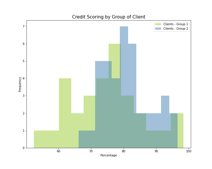
E.直方图 (E. Histogram)

A histogram tells us how many values in a dataset fall between different sets of numbers, for example how many numbers fall between 0 and 10? This question represents a bin which might be between 0 and 10.

直方图告诉我们数据集中有多少个值落在不同的数字集之间，例如有多少个数字落在0到10之间？ 这个问题代表一个bin，可能在0到10之间。

All bins in a histogram are always the same size:

直方图中的所有bin大小始终相同：

• The width of each bin is the distance between the minimum and maximum values of each bin.

  每个仓的宽度是每个仓的最小值和最大值之间的距离。

• Each bin is represented by a different rectangle whose height is the number of elements from the dataset that fall within that bin.

  每个容器由一个不同的矩形表示，其高度是数据集中属于该容器的元素数。

The command plt.hist finds the minimum and the maximum values in your dataset and creates 10 equally-spaced bins between those values by default. If we want more than 10 bins, we can use the keyword bins to set the instruction.

命令plt.hist在数据集中查找最小值和最大值，并默认在这些值之间创建10个等距的bin。 如果我们要使用10个以上的容器，则可以使用关键字容器来设置指令。

A problem we face is that our histograms might have different numbers of samples, making one much bigger than the other. To solve this, we can normalize our histograms using normed=True.

我们面临的一个问题是，直方图可能具有不同数量的样本，使得一个样本比另一个样本大得多。 为了解决这个问题，我们可以使用normed = True标准化直方图。

In the example below, I include a credit scoring case in which we want to visualize how scores are distributed among both groups of clients. I tailored the histogram to create 12 bins instead of the default 10 and to set alpha or transparency level at 0.5 in order to see both histograms at the same time avoiding overlapping distributions.

在下面的示例中，我包括一个信用评分案例，在该案例中，我们希望可视化如何在两组客户之间分配分数。 我调整了直方图，以创建12个bin而不是默认的10个bin，并将alpha或透明度级别设置为0.5，以便同时查看两个直方图，避免重叠分布。

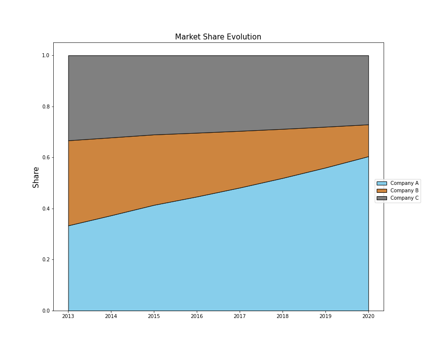
F.堆积图 (F. Stacked Plot)

This type of chart plots the variables of a table or timetable in a stacked plot, up to a maximum of 25 variables. The function plots the variables in separate y-axes, stacked vertically. The variables share a common x-axis.

这种类型的图表以堆积图的形式绘制表或时间表的变量，最多25个变量。 该函数将变量绘制在垂直堆叠的单独y轴中。 变量共享一个公共的x轴。

I’m going to simulate the case of the evolution of market share for three companies for the last eight years, with the respective visualization in the stacked plot:

我将模拟过去八年中三家公司的市场份额演变情况，并在堆叠图中分别显示：

 # Insert DataFrames:
year = pd.DataFrame(range(2013,2021),columns=['Year'])
volume1 = pd.DataFrame([1000,1100,1200,1250,1300,1350,1400,1450], columns=['Values 1'])
volume2 = pd.DataFrame([1000,900,800,700,600,500,400,300], columns=['Values 2'])
volume3 = pd.DataFrame([1000,950,900,850,800,750,700,650], columns=['Values 3']) # Create main frame:
frames = [year,volume1, volume2, volume3]
frame = pd.concat(frames,axis=1) # Plot axis, labels, colors:
x_values = frame['Year']
y_values = np.vstack([frame['Values 1'], frame['Values 2'], frame['Values 3']])
labels = ['Company A', 'Company B', 'Company C']
colors = ['skyblue', 'peru', 'gray'] # Display plot:
fig = plt.figure(figsize=(10,8))
plt.stackplot(x_values, y_values, labels=labels, colors=colors ,edgecolor='black')
plt.title('Market Share Evolution',fontsize=15)
plt.ylabel('Share', fontsize=15)
plt.legend(loc='best')
plt.show()

G.百分比堆积图 (G. Percentage Stacked plot)

Also known as a 100% Stacked Area Chart, this chart displays the trend of the percentage each value contributes over time or categories.

也称为100％堆积面积图，此图显示每个值在时间或类别中所占百分比的趋势。

In this case, we’ll plot the same information as in the Stacked Plot but with the percentage contributed to the total market share by each company:

在这种情况下，我们将绘制与堆积图相同的信息，但百分比对每个公司的总市场份额有所贡献：

结论 (Conclusion)

With the posted guidelines and plot types in this article, I hope to have helped you to enhance your data analytics skills, at least from a data-visualization stand point.

希望借助本文中发布的指南和绘图类型，至少从数据可视化的角度来看，希望能帮助您提高数据分析技能。

This is the beginning of a series of articles related to data-visualization that I’ll be preparing to share more insights and knowledge. If you liked the information included in this article don’t hesitate to contact me to share your thoughts. It motivates me to keep on sharing!

这是与数据可视化相关的一系列文章的开始，我将准备分享更多的见解和知识。 如果您喜欢本文中包含的信息，请随时与我联系以分享您的想法。 这激励着我继续分享！

Thanks for taking the time to read my article! Any question, suggestion or comment, feel free to contact me: herrera.ajulian@gmail.com

感谢您抽出宝贵的时间阅读我的文章！ 如有任何问题，建议或意见，请随时与我联系：herrera.ajulian@gmail.com

翻译自: https://towardsdatascience.com/business-intelligence-visualizations-with-python-1d2d30ce8bd9

python可视化