python 探索性分析_python中的探索性文本分析

python 探索性分析

Why do we do exploratory data analysis before we build a model? I would say ‘to understand the data better so that we preprocess the data in a suitable way and choose an appropriate modelling technique’. This necessity to understand data is still relevant when working with text data. This post is the first of the three sequential articles on steps to build a sentiment classifier. In this post, we will look at one way to conduct exploratory data analysis on text, or exploratory text analysis for brevity.

为什么要在建立模型之前进行探索性数据分析？ 我会说“ 更好地理解数据，以便我们以合适的方式预处理数据并选择合适的建模技术” 。 在处理文本数据时，理解数据的必要性仍然很重要。 这篇文章是有关建立情感分类器的三篇连续文章的第一篇。 在本文中，我们将探讨一种对文本进行探索性数据分析或为简洁起见进行探索 性文本分析的方法。

Before we dive in, let’s take a step back and look at the bigger picture first. CRISP-DM methodology outlines the process flow for a successful data science project. In the diagram below, 2–4th stages of data science project are shown. In data understanding stage, exploratory data analysis is one of the key tasks.

在我们深入之前，让我们退后一步，先看看大图。 CRISP-DM方法论概述了成功的数据科学项目的流程。 在下图中，显示了数据科学项目的第2至第4阶段。 在数据理解阶段，探索性数据分析是关键任务之一。

Extract from CRISP-DM process flow

摘自CRISP-DMCraft.io流程

When working on a data science project, it is not unusual to be going back and forth between stages rather than linearly progressing. This is because ideas and questions come up in subsequent stages and you want to go back a stage or two to try out the idea or find the answer to the question. The pink arrows are not in the official CRISP-DM, however, I think these are often necessary. In fact, we will be doing a bit of data preparation in this post for the purpose of exploratory text analysis. For those who are interested to learn more about CRISP-DM, this is a nice short introduction and this resource provides a more detailed explanation.

在进行数据科学项目时，通常在阶段之间来回移动而不是线性进行。 这是因为想法和问题会在随后的阶段出现，并且您想回到一两个阶段来尝试想法或找到问题的答案。 粉色箭头不在官方的CRISP-DM中，但是，我认为这些经常是必要的。 实际上，出于探索性文本分析的目的，我们将在本文中做一些数据准备。 对于那些有兴趣了解CRISP-DM的人来说， 这是一个不错的简短介绍，并且本资源提供了更详细的说明。

0. Python设置🔧 (0. Python setup 🔧)

This post assumes that the reader (👀 yes, you!) has access to and is familiar with Python including installing packages, defining functions and other basic tasks. If you are new to Python, this is a good place to get started.

这篇文章假定读者(👀，是的，您！)可以访问并熟悉Python，包括安装软件包，定义函数和其他基本任务。 如果您不熟悉Python，那么这是一个入门的好地方。

I have tested the scripts in Python 3.7.1 in Jupyter Notebook.

我已经在Jupyter Notebook中的Python 3.7.1中测试了脚本。

Let’s make sure you have the following libraries installed before we start:◼️ Data manipulation/analysis: numpy, pandas◼️ Data partitioning: sklearn◼️ Text preprocessing/analysis: nltk◼️ Visualisation: matplotlib, seaborn

让我们确保你已经在我们开始之前安装以下库：◼️ 数据处理/分析：numpy 的，熊猫 ◼️ 数据分区：sklearn◼️ 文本预处理/分析：NLTK Visual️ 可视化： matplotlib，seaborn

Once you have nltk installed, please make sure you have downloaded ‘punkt’, ‘stopwords’ and ‘wordnet’ from nltk with the script below:

一旦安装了nltk ，请确保使用以下脚本从nltk下载了“ punkt” ， “ stopwords ”和“ wordnet” ：

import nltk
nltk.download('punkt') # for sent_tokenize
nltk.download('stopwords') 
nltk.download('wordnet') # for WordNetLemmatizer

If you have already downloaded, running this will notify you of so.

如果您已经下载了，运行它会通知您。

Now, we are ready to import all the packages:

现在，我们准备导入所有软件包：

# Setting random seed
seed = 123# Data manipulation/analysis
import numpy as np
import pandas as pd# Data partitioning
from sklearn.model_selection import train_test_split# Text preprocessing/analysis
import re
from nltk import word_tokenize, sent_tokenize, FreqDist
from nltk.util import ngrams
from nltk.corpus import stopwords
from nltk.stem import WordNetLemmatizer
from nltk.tokenize import RegexpTokenizer# Visualisation
import matplotlib.pyplot as plt
%matplotlib inline
import seaborn as sns
sns.set(style="whitegrid", context='talk')

Takeaways or notes will be accompanied with 🍀 when exploring.

游览时， 外卖品或笔记会附带 🍀。

1.数据📦 (1. Data 📦)

We will use IMDB movie reviews dataset. You can download the dataset here and save it in your working directory. Once saved, let’s import it to Python:

我们将使用IMDB电影评论数据集。 您可以在此处下载数据集并将其保存在您的工作目录中。 保存后，让我们将其导入Python：

sample = pd.read_csv('IMDB Dataset.csv')
print(f"{sample.shape[0]} rows and {sample.shape[1]} columns")
sample.head()

From looking at the head of the data, we can instantly see that there are html tags in the second record.

通过查看数据的开头，我们可以立即看到第二条记录中有html标签。

🍀 Inspect html tags further and see how prevalent they are.

further 进一步检查html标签，看看它们的流行程度。

Let’s look at the split between sentiments:

让我们看一下情感之间的分歧：

sample['sentiment'].value_counts()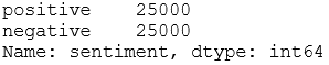

Sentiment is evenly split in the sample data. Before we start exploratory text analysis, let’s first partition the data into two sets: train and test. We will set aside 5000 cases for testing:

情感在样本数据中平均分配。 在开始探索性文本分析之前，让我们首先将数据分为两组： train和test 。 我们将预留5000个案例进行测试：

# Split data into train & test
X_train, X_test, y_train, y_test = train_test_split(sample['review'], sample['sentiment'], test_size=5000, random_state=seed, 
                                                    stratify=sample['sentiment'])# Append sentiment back using indices
train = pd.concat([X_train, y_train], axis=1)
test = pd.concat([X_test, y_test], axis=1)# Check dimensions
print(f"Train: {train.shape[0]} rows and {train.shape[1]} columns")
print(f"{train['sentiment'].value_counts()}\n")print(f"Test: {test.shape[0]} rows and {test.shape[1]} columns")
print(test['sentiment'].value_counts())

By specifying the stratify argument, we ensured that sentiment is evenly split in both sets.

通过指定stratify参数，我们确保将情感平均分配到两组中。

We will be using train for the exploratory text analysis in this post. Once we explore the training dataset, it may be useful to check the key characteristics of test set separately. Ideally, both sets should be representative of the underlying population. Let’s inspect the head of the training dataset:

在这篇文章中，我们将使用Train进行探索性文本分析。 一旦我们探索了训练数据集，单独检查测试集的关键特征可能会很有用。 理想情况下，两组都应代表基础人口。 让我们检查训练数据集的头部：

train.head()

Alright, we are all set to explore! ✨

好了，我们都准备探索！ ✨

2.探索性文本分析analysis (2. Exploratory text analysis 🔎)

One way to guide exploratory data analysis is to write down questions that you are interested in and answer them with the data. Finding answers to questions often leads to other questions that you may want to explore. Here are some example questions we could answer:

指导探索性数据分析的一种方法是写下您感兴趣的问题并用数据回答。 找到问题的答案通常会导致您可能想探索其他问题。 以下是一些我们可以回答的示例问题：

📋 2.1. Warm-up:* How many strings are there?* What are the most common strings?* How do the shortest strings look like?* How do the longest strings look like?

📋2.1 。 热身： *有多少个字符串？*最常见的字符串是什么？*最短的字符串看起来如何？*最长的字符串看起来如何？

📋 2.2. Tokens:

📋2.2 。 代币：

💡 Token is a sequence of characters. Tokens are often loosely referred to as words.💡 Tokenisation is a process of splitting a document into tokens and sometimes also throwing away certain characters such as punctuation. Example: Tokenisation turns ‘This movie was awesome’ into 4 tokens: [‘This’, ‘movie’, ‘was’, ‘awesome’]

💡 令牌是一个字符序列。 令牌通常被简称为单词。 💡 令牌化是将文档拆分为令牌的过程，有时还会丢弃某些字符，例如标点符号。 示例：令牌化将“这部电影很棒”转换为4个令牌：['This'，'movie'，'was'，'awesome']

* How many tokens are there?* How many unique tokens are there?* What is the average number of characters per token?

*有多少令牌？*有多少唯一令牌？*每个令牌的平均字符数是多少？

📋 2.3. Stop words:

📋2.3 。 停用词：

💡 Stop words are common words which provide little to no value to the meaning of the text. Example: the, a, and.

💡停用词是常用词，对文本的含义几乎没有价值。 示例：a，a和。

* What are the most common stop words?* What other words occur so often such that could be added to stop words?

*最常见的停用词是什么？*经常出现哪些其他词，可以将其添加到停用词中？

📋 2.4. Common word n-grams:

📋2.4 。 常用字n-gram：

💡 Word n-grams are all combinations of adjacent n words in text data. Example: Bigrams in ‘This movie was awesome’ are [‘This movie’, ‘movie was’, ‘was awesome’]

💡 字的n-gram在文本数据相邻的n个字的所有组合 。 例如：“这部电影真棒”中的Bigrams是[“这部电影”，“电影是”，“真棒”]

* What are the most common tokens?* What are the most common bigrams?* What are the most common trigrams?* What are the most common fourgrams?

*最常见的标记是什么？*最常见的双字母是什么？*最常见的三字母组合是什么？*最常见的四字母组合是什么？

📋 2.5. Documents:

📋2.5 。 文件：

💡 Document is a text record. Example: each movie review is a document.💡 Corpus is a collection of documents. Simply put, text data is a corpus. Example: we can refer training data as training corpus.

💡文档是文本记录。 示例：每个电影评论都是一个文档。 💡语料库是文件的集合。 简而言之，文本数据是语料库。 示例：我们可以将训练数据称为训练语料库。

* What is the average number of sentences per document?* What is the average number of tokens per document?* What is the average number of characters per document?* What is the average number of stop words per document?* How do the answers differ by sentiment?

*每个文档的平均句子数是多少？*每个文档的平均标记数是多少？*每个文档的平均字符数是多少？*每个文档的平均停用词数是多少？*答案如何情绪有所不同？

Now, it’s time to find answers to these questions! 😃

现在，是时候找到这些问题的答案了！ 😃

📋2.1。 W 准备 (📋 2.1. Warm-up)

Let’s merge all the reviews into one string and then split it into sub-strings (here onward referred to as strings) on white space. This ensures the corpus is minimally altered (e.g. keeping punctuation as it is) for this warm-up exploration:

让我们将所有评论合并到一个字符串中，然后在空白处将其拆分为子字符串(此处称为字符串)。 这样可以确保在此热身探索中，语料库的变化最小(例如，保持标点符号不变)：

# Prepare training corpus into one giant string
train_string = " ".join(X_train.values)
print(f"***** Extract of train_string ***** \n{train_string[:101]}", "\n")# Split train_corpus by white space
splits = train_string.split()  
print(f"***** Extract of splits ***** \n{splits[:18]}\n")

✏️ 2.1.1. How many strings are there?

2.1️2.1.1 。 有多少个琴弦？

print(f"Number of strings: {len(splits)}")
print(f"Number of unique strings: {len(set(splits))}")

There are over 10 million strings in the training corpus with around 410 thousand unique strings. This gives us initial ballpark figures. We will get a view on how these numbers look for tokens after we tokenise properly.

训练语料库中有超过1000万个字符串，其中约有41万个唯一字符串。 这给了我们初步的数字。 在正确标记后，​​我们将了解这些数字如何寻找标记。

✏️ 2.1.2. What are the most common strings?

2.1️2.1.2 。 最常见的字符串是什么？

Let’s prepare frequency distribution for each string to answer the question:

让我们为每个字符串准备频率分布以回答问题：

freq_splits = FreqDist(splits)
print(f"***** 10 most common strings ***** \n{freq_splits.most_common(10)}", "\n")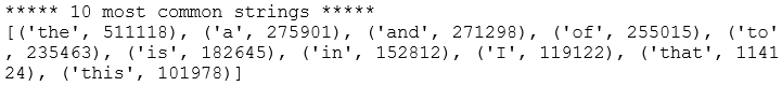

It is not surprising to see that most common strings are stop words. We will explore stop words further later in section 2.3. Stop words.

看到最常见的字符串是停用词就不足为奇了。 我们将在第2.3节中进一步探讨停用词。 停词 。

🍀 Remove stop words before looking at common tokens and n-grams.

looking 在查看常见标记和n-gram之前，请删除停用词。

✏️ 2.1.3. How do the shortest strings look like?

2.1️2.1.3。 最短的弦长如何？

Let’s define short string as strings with a length of less than 4 characters and check their frequency:

让我们将短字符串定义为长度少于4个字符的字符串，并检查其频率：

short = set(s for s in splits if len(s)<4)
short = [(s, freq_splits[s]) for s in short]
short.sort(key=lambda x:x[1], reverse=True)
short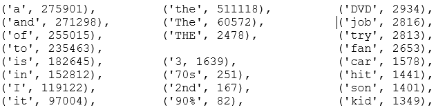

extract from short , not all outputs are shown

从 short中 摘录 ，未显示所有输出

Many short strings appear to be stop words but there are also numbers and other short words.

许多短字符串似乎是停用词，但也有数字和其他短词。

🍀 There are numbers in different forms: 3, 2nd, 70s, 90% — we need to decide whether to drop or keep them.

numbers 有不同形式的数字： 3、2、70、90 ％-我们需要决定是否丢弃或保留它们。

🍀 There is case variation: ‘the’, ‘The’, ‘THE’ - these need to be normalised.

case 存在大小写差异：'the'，'The'，' THE'- 这些需要标准化。

Because we haven’t tokenised yet, some strings currently contain punctuation that is attached to a word. As a result, otherwise same words are considered as different as shown in this example:

由于我们尚未标记符号，因此某些字符串当前包含附加到单词的标点符号。 结果，如以下示例所示，相同的单词被认为是不同的：

extract from short , not all outputs are shown

从 short中 摘录 ，未显示所有输出

🍀 Discarding punctuation will be helpful to further normalise words.

🍀丢弃标点符号将有助于进一步规范单词。

✏️ 2.1.4. How do the longest strings look like?

2.️2.1.4。 最长的弦长如何？

Let’s define long strings as 16+ characters long and repeat the process.

让我们将长字符串定义为16个以上的字符，然后重复该过程。

long = set(s for s in splits if len(s)>15)
long = [(s, freq_splits[s]) for s in long]
long.sort(key=lambda x:x[1], reverse=True)
long

extract from long , not all outputs are shown

从 long中 提取 ，未显示所有输出

The frequency of long string looks much lower than short strings which is not too surprising. Long strings look quite interesting and there are a few key takeaways:

长字符串的频率看起来比短字符串的频率低得多，这并不奇怪。 长字符串看起来很有趣，并且有一些关键要点：

🍀 There is American and British spelling of the same word: ‘characterization’ vs ‘characterisation’. After a quick check using the script below, American spelling looks more dominant for this word. Quantifying how prevalent the two spelling in the entire training corpus is a bit tricky.

American美国和英国的同一个单词拼写为：“字符化”与“字符化”。 在使用下面的脚本快速检查后，该单词的美国拼写看上去更占优势。 量化这两个拼写在整个训练语料库中的流行程度有些棘手。

print(f"characterisation: {sum([c for s, c in long if re.match(r'characterisation*', s.lower())])} strings")
print(f"characterization: {sum([c for s, c in long if re.match(r'characterization*', s.lower())])} strings")

🍀 There are hyphenated words: ‘thought-provoking’, ‘post-apocalyptic’, ‘under-appreciated’ and ‘film--specially’ (this one with double hyphens). If we tokenise on white space or punctuation, these strings will be split into separate words. For most cases, this will conserve the gist of the sentence. If we keep hyphenated words as they are, they won’t be as common and consequently removed as rare words.

hy 有连字词：“发人深省”，“后世界末日”，“欣赏不足”和“特别是电影”(这个带有双连字符)。 如果我们在空白或标点符号上标记，则这些字符串将被拆分为单独的单词。 在大多数情况下，这将保留句子的要旨。 如果我们保留连字符的原样，它们将不会像普通字一样普遍，因此会被删除。

🍀 There are words combined with other punctuation (some due to lack of space): ‘actors/actresses’, ‘Mission:Impossible’, “actors(HA!HA!HA!)…they’re”, ‘different:actually,Bullock’. It would be good to separate these cases into separate words when tokenising. So probably tokenising based on white space or punctuation is a good idea.

🍀 有些单词加上其他标点符号(有些是由于篇幅所致) ：“ 演员/女演员”，“任务：不可能”，“演员(HA！HA！HA！)……他们”，“不同：实际上，犍'。 在标记时，最好将这些情况分成单独的单词。 因此，基于空白或标点的标记可能是一个好主意。

🍀 There are websites and email addresses: ‘/>www.ResidentHazard.com’, ‘http://www.PetitionOnline.com/gh1215/petition.html’, ‘IAMASEAL2@YAHOO.COM’’. However, there doesn’t seem to be many.

🍀 有网站和电子邮件地址： “ />”。www.ResidentHazard.com”， “ http://www.PetitionOnline.com/gh1215/petition.html”、“IAMASEAL2@YAHOO.COM”。 但是，似乎并不多。

🍀 There are outlaw words that repeats the same character more than twice: “Booooring…….Don’t”, ‘NOOOOOOIIIISE!),’. If you know the correct term for these elongated words, I would love to find out. Until then, we will refer them as ‘outlaw words’. These outlaw cases seem to appear very rarely.

🍀 有些不合法的单词会重复同一字符两次以上 ： “ Booooring…….Don't”，“ NOOOOOOIIIISE！)”。 如果您知道这些拉长单词的正确术语，我很想找出答案。 在此之前，我们将其称为“违法用语”。 这些违法案件似乎很少出现。

There are other interesting findings we could add to these but these are good starters for now.

我们还可以添加其他有趣的发现，但是目前这些都是很好的入门。

It’s important to understand whether these cases that we just explored are prevalent enough to justify additional preprocessing steps (i.e. longer run time). It’s useful to experiment to see if adding an additional preprocessing step improves model performance. We will do a bit of this in the third post.

重要的是要了解我们刚刚探讨的这些案例是否足够普遍以证明其他预处理步骤(即更长的运行时间)是合理的。 尝试查看是否添加额外的预处理步骤可以提高模型性能，这很有用。 我们将在第三篇文章中对此做一些说明。

✏️ 2.1.5. Following up questions emerged so far

2.️2.1.5。 迄今为止出现了后续问题

We have answered all 4 warm up questions! While looking for answers, we have gathered even more questions. Before we jump to the next set of predefined questions, let’s quickly follow up some of the questions that have came up on the go.

我们已经回答了所有4个热身问题！ 在寻找答案的同时，我们收集了更多的问题。 在跳到下一组预定义的问题之前，让我们快速跟进旅途中出现的一些问题。

◼️ How frequent is html tags? This question emerged when we were looking at head of the sample data in section 1. Data. The example html tag: ‘<br /><br />’ would have been split into three strings: ‘<br’, ‘/><br’ and ‘/>’ when we split the data based on white space. On side note, the <br> tag seems to be used to break lines. Let’s roughly gauge how prevalent the html tags are.

◼️html 标签的频率是多少？ 当我们在第1节“数据”中查看样本数据的开头时，出现了这个问题。 当我们根据空格分割数据时，示例html标签：“ <br /> <br />”将被拆分为三个字符串：“ <br”，“ /> <br”和“ />”。 附带说明， <br>标签似乎用于换行。 让我们大致评估一下html标签的流行程度。

All follow up questions are similar since we are going to assess the frequency of a particular type of string. To avoid repeating ourselves, let’s make a function.

所有后续问题都类似，因为我们将评估特定类型的字符串的频率。 为了避免重复自己，让我们做一个函数。

def summarise(pattern, strings, freq):
    """Summarise strings matching a pattern."""
    # 1. Find matches
    compiled_pattern = re.compile(pattern)
    matches = [s for s in strings if compiled_pattern.search(s)]
    # 2. Print volume and proportion of matches
    print("{} strings, that is {:.2%} of total".format(len(matches), len(matches)/ len(strings)))
    # 3. Create list of tuples containing matches and their frequency
    output = [(s, freq[s]) for s in set(matches)]
    output.sort(key=lambda x:x[1], reverse=True)
    return output# Find strings possibly containing html tag
summarise(r"/?>?w*<|/>", splits, freq_splits)

not all outputs are shown

并非所有输出都显示

If we scroll through the output, there aren’t many html tags other than the <br> tag and a few cases of <i> tag.

如果我们滚动浏览输出，除了<br>标记和<i>标记的少数情况之外，没有太多的html标记。

🍀 If we remove punctuation when tokenising, ‘/><br’ and ‘<br’ will become ‘br’ and we could probably add ‘br’ to stop words.

🍀 如果在标记词时删除标点符号，则'/> <br'和'<br'将变为'br'，我们可能会添加'br'来停止单词。

◼ ️How frequent are numbers? We found some instances of numbers from section 2.1.3. Short strings. Let’s see how frequent they are with the following script:

◼️数字有多频繁？ 我们从2.1.3节中找到了一些数字实例。 短弦 。 让我们看看使用以下脚本的频率：

summarise(r"\d", splits, freq_splits)

not all outputs are shown

并非所有输出都显示

Strings containing numbers are infrequent. In the context of movie reviews, it’s hard to intuitively make sense of how numbers would be useful. 10/10 could be an indication of positive sentiment but what can we infer from numbers such as 4, 80’s and 20th? We will drop numbers when tokenising.

包含数字的字符串很少见。 在电影评论的背景下，很难直观地理解数字将如何有用。 10/10可能表示积极情绪，但是我们可以从数字(例如4、80和20)推断出什么呢？ 标记时，我们将删除数字。

Depending on the timeline of a project, you may not have enough time to try all the interesting ideas. In that case, it’s handy to keep a list of nice-to-try items which you could experiment with when you have time. We will add the following tasks to that list: 1) Keep and convert numbers to text2) Create a feature indicating whether a review contains numbers or not

根据项目的时间表，您可能没有足够的时间来尝试所有有趣的想法。 在这种情况下，保留一份易于尝试的项目列表是很方便的，您可以在有空的时候进行尝试 。 我们将在该列表中添加以下任务：1)保存数字并将其转换为文本2)创建一个功能，指示评论中是否包含数字

◼ ️How frequent are hyphenated words? We saw hyphenated words when inspecting long strings in section 2.1.4.Let’s see how frequent they are:

️️连字词的频率是多少？ 在第2.1.4节中检查长字符串时，我们看到了带连字符的单词。让我们看看它们有多频繁：

summarise(r"\w+-+\w+", splits, freq_splits)

not all outputs are shown

并非所有输出都显示

Roughly less than 1% of strings contained hyphenated words. From glancing through the hyphenated words, it makes more sense to separate them out to keep the data simple. For example: We should tokenise ‘camera-work’ to 2 tokens: [‘camera’, ‘work’] instead of 1 token: [‘camera-work’]. We could add ‘keep hyphenated words as they are’ to the list of nice-to-try items.

大约不到1％的字符串包含带连字符的单词。 从扫视连字符开始的单词，将它们分开以保持数据简单更有意义。 例如：我们应该将'camera-work'标记为2个标记：['camera'，'work']而不是1个标记：['camera-work']。 我们可以将“保留带连字符的单词原样”添加到易于尝试的项目列表中。

◼ ️How frequent are words combined by other punctuation? Much like the previous question, we saw these cases during long string exploration. Let’s see how frequent they are:

️️单词被其他标点符号组合的频率是多少？ 就像前面的问题一样，我们在长字符串探索中看到了这些情况。 让我们看看它们的频率：

summarise(r"\w+[_!&/)(<\|}{\[\]]\w+", splits, freq_splits)

not all outputs are shown

并非所有输出都显示

Not too frequent, these ones definitely need to be separated.

不太频繁，这些绝对一定要分开。

◼ ️How frequent are outlaw words? We saw elongated words like ‘NOOOOOOIIIISE!),’ earlier. Let’s see how prevalent they are:

◼️不合法的单词多久出现一次？ 之前我们看到过一些拉长的字眼，例如“ NOOOOOOIIIISE！)。 让我们看看它们有多普遍：

def find_outlaw(word):
    """Find words that contain a same character 3+ times in a row."""
    is_outlaw = False
    for i, letter in enumerate(word):
        if i > 1:
            if word[i] == word[i-1] == word[i-2] and word[i].isalpha():
                is_outlaw = True
                break
    return is_outlawoutlaws = [s for s in splits if find_outlaw(s)]
print("{} strings, that is {:.2%} of total".format(len(outlaws), len(outlaws)/ len(splits)))
outlaw_freq = [(s, freq_splits[s]) for s in set(outlaws)]
outlaw_freq.sort(key=lambda x:x[1], reverse=True)
outlaw_freq

not all outputs are shown

并非所有输出都显示

These are not worth correcting for because there too few cases.

这些不值得纠正，因为案例太少了。

That was the last follow up question! We have learned a little bit about the data. Hope you are feeling warmed up. 💦 You may have noticed how easily we could keep expanding our questions and keep exploring? In the interest of time, we will stop this section here and try to keep the next sections as succinct as possible. Otherwise, this post will be over a few hours long. 💤

那是最后的跟进问题！ 我们已经了解了一些数据。 希望你感到热身。 💦您可能已经注意到我们可以轻松扩展问题并继续探索吗？ 为了节省时间，我们将在这里停止本节，并尝试使下一节尽可能简洁。 否则，该帖子将持续几个小时。 💤

📋2.2。 代币 (📋 2.2. Tokens)

Let’s answer these two questions at one go:

让我们一次性回答以下两个问题：

✏️ 2.2.1. How many tokens are there?✏️ 2.2.2. How many unique tokens are there?

2.2️2.2.1 。 有多少代币？ 2.2️2.2.2 。 有多少个唯一令牌？

We have to tokenise the data first. Recalling from earlier exploration, it seemed best to drop punctuation and numbers when tokenising. With this in mind, let’s tokenise the text into alphabetic tokens:

我们必须首先标记数据。 回顾先前的研究，在标记化时最好删除标点符号和数字。 考虑到这一点，让我们将文本标记为字母标记：

tokeniser = RegexpTokenizer("[A-Za-z]+")
tokens = tokeniser.tokenize(train_string)
print(tokens[:20], "\n")

Now we have tokenised, we can answer the first two questions:

现在我们有了标记，我们可以回答前两个问题：

print(f"Number of tokens: {len(tokens)}")
print(f"Number of unique tokens: {len(set(tokens))}")

There are over 10 million tokens in the training data with around 122 thousand unique tokens. Currently, ‘Watch’, ‘watch’ and ‘watching’ are counted as different tokens. Hmm, wouldn’t it be great if we could normalise them to ‘watch’ and count them as one unique token? If we normalise, the number of unique tokens would be lower. Let’s quickly do two things: convert all tokens into lowercase and lemmatise them:

训练数据中有超过1000万个令牌，其中约有122,000个唯一令牌。 当前，“监视”，“监视”和“监视”被视为不同的令牌。 嗯，如果我们可以将它们标准化为“监视”并将其视为一个唯一令牌，那不是很好吗？ 如果我们归一化，唯一令牌的数量将会减少。 让我们快速地做两件事：将所有标记转换为小写并对其进行定理：

lemmatiser = WordNetLemmatizer()
tokens_norm = [lemmatiser.lemmatize(t.lower(), "v") for t in tokens]
print(f"Number of unique tokens: {len(set(tokens_norm))}")

Great, the number of unique tokens dropped by about 30%.

太好了，独特代币的数量下降了约30％。

📌 Exercise: If you are keen and have time, instead of combining both steps like above, try separating out and see how the number of unique tokens change at each step. For instance, you could first convert tokens to lowercase, and check the number, and then lemmatise and check the number again. If you change the order of these two operations, is the final number of unique tokens different than 82562? Why would that be?

📌练习：如果您渴望并且有时间，不要像上面那样将两个步骤组合在一起，而是试着分开看看每个步骤中唯一令牌的数量如何变化。 例如，您可以先将令牌转换为小写字母，然后检查数字，然后进行词法修饰并再次检查数字。 如果更改这两个操作的顺序，唯一令牌的最终数量是否不同于82562？ 为什么会这样呢？

👂 Psst, I will show another way to lemmatise in the next post when preprocessing the text for the model.

s 抱歉， 在下一篇文章中， 当预处理模型文本时 ，我将展示另一种词法定理 。

✏️ 2.2.3. What is the average number of characters per token?

2.2️2.2.3 。 每个令牌的平均字符数是多少？

Let’s find out the average token length and inspect its the distribution:

让我们找出平均令牌长度并检查其分布：

# Create list of token lengths for each token
token_length = [len(t) for t in tokens]# Average number of characters per token
print(f"Average number of characters per token: {round(np.mean(token_length),4)}")# Plot distribution
plt.figure(figsize=(12, 12))
sns.countplot(y=token_length)
plt.title("Counts of token length", size=20);

There are a few tokens that is very long but also very rare. Let’s look at the exact counts for those longer than 10 characters:

有一些令牌很长，但也很罕见。 让我们看一下那些超过10个字符的确切计数：

pd.DataFrame(data=token_length, columns=['length']).query("length>10").value_counts()

17+ characters long words are infrequent. Let’s inspect some of them:

不超过17个字符的长单词。 让我们检查其中的一些：

[t for t in tokens if len(t)>=20]

not all outputs are shown

并非所有输出都显示

Interesting, some are valid long words whereas some are long because they lack white space or outlaw words (i.e. elongated).

有趣的是，有些是有效的长字，而有些则是长字，因为它们缺少空格或非法字(即加长)。

🍀 When preprocessing, we should make sure that very rare tokens like these ones are dropped such that they won’t create separate columns when vectorising tokens into a matrix.

processing 进行预处理时，我们应确保丢弃诸如此类这样的非常稀有的标记，以便在将标记矢量化为矩阵时不会创建单独的列。

📋2.3。 停用词 (📋 2.3. Stop words)

✏️ 2.3.1. What are the most frequent stop words?

2.3️2.3.1 。 最常用的停用词是什么？

Let’s first inspect all stop words:

让我们首先检查所有停用词：

stop_words = stopwords.words("english")
print(f"There are {len(stop_words)} stopwords.\n")
print(stop_words)

At the time of writing this post, there are 179 stop words. The list of stop words could extend in future. It appears that we could extend the stop words to include a few more. In fact, I have proposed on Github to add generic stop words from below to the list of English stop words in nltk. Let’s also make sure to add a custom stop word ‘br’ to the list:

在撰写本文时，有179个停用词。 停用词列表可能会在将来扩展。 看来我们可以将停用词扩展到更多。 实际上，我已经在Github上建议将以下通用停用词添加到nltk中的英语停用词列表中。 我们还要确保添加自定义停用词“ br” 到列表：

stop_words.extend(["cannot", "could", "done", "let", "may" "mayn",  "might", "must", "need", "ought", "oughtn", "shall", "would", "br"])
print(f"There are {len(stop_words)} stopwords.\n")

Now, let’s check what are the most common stop words:

现在，让我们检查最常见的停用词：

freq_stopwords = [(sw, tokens_norm.count(sw)) for sw in stop_words]
freq_stopwords.sort(key=lambda x: x[1], reverse=True)
freq_stopwords[:10]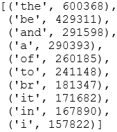

The frequency is really high (duh, I mean they are stop words, of course they will be frequent 😈), especially for ‘be’ and ‘the’. Wouldn’t it be interesting to find out what proportion of tokens are stop words? Let’s quickly check:

频率确实很高(high，我是说它们是停用词，当然它们会经常出现)，尤其是对于“ be”和“ the”。 找出停用词占代币的比例是不是很有趣？ 让我们快速检查一下：

n_stopwords = len([t for t in tokens_norm if t in stop_words])
print(f"{n_stopwords} tokens are stop words.")
print(f"That is {round(100*n_stopwords/len(tokens_norm),2)}%.")

About half of the tokens are stop words. 💭

大约一半的标记是停用词。 💭

✏️2.3.2. What other words occur so often such that could be added to stop words?

2.3️2.3.2 。 还有哪些其他单词经常出现，可以添加到停用词中？

We will answer this question when we look at common tokens soon.

当我们很快查看通用令牌时，我们将回答这个问题。

📋2.4。 普通n元 (📋 2.4. Common n-grams)

It’s time to find out common n-grams. Let’s answer all four questions together:

是时候找出常见的n-gram了。 让我们一起回答所有四个问题：

✏️ 2.4.1–4. What are the most common tokens, bigrams, trigrams and fourgrams?

2.️2.4.1–4。 什么是最常见的令牌，二元组，三元组和四元组？

Firstly, let’s remove stop words:

首先，让我们删除停用词：

tokens_clean = [t for t in tokens_norm if t not in stop_words]
print(f"Number of tokens: {len(tokens_clean)}")

This is the remaining 49% of tokens. Now, we can inspect the common tokens (i.e. unigrams), bigrams, trigrams and fourgrams:

这是令牌的剩余49％。 现在，我们可以检查常见的标记(即unigram)，bigrams，trigram和fourgrams：

def get_frequent_ngram(tokens, ngram, n=20):
    """Find most common n n-grams in tokens."""
    n_grams = ngrams(tokens, ngram)
    freq_dist = FreqDist(n_grams)
    top_freq = freq_dist.most_common(n)
    return pd.DataFrame(top_freq, columns=["ngram", "count"])# Get frequent ngrams for all 4
for i in range(1,5):
    mapping = {1:"uni", 2:"bi", 3:"tri", 4:"four"}
    plt.figure(figsize=(12,10))
    sns.barplot(x="count", y="ngram", data=get_frequent_ngram(tokens_clean, i))
    plt.title(f"Most common {mapping[i]}grams");

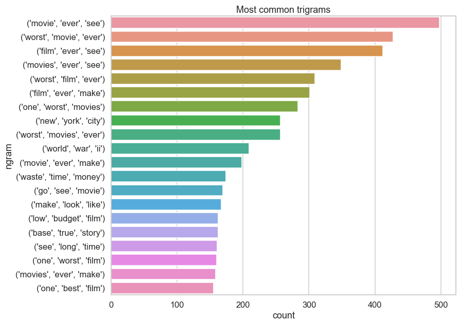
The word ‘film’ and ‘movie’ looks quite frequent compared to the other frequent words. The answer to question 2.3.2. is to potentially add ‘movie’, and ‘film’ to stop words. It’s interesting to see frequent bigrams, trigrams and fourgrams. As we increase n, the frequency drops as expected. Bigrams may be potentially useful but trigrams and fourgrams are not frequent enough relative to the token frequency.

与其他常用词相比，“电影”和“电影”这个词看起来很常见。 问题2.3.2的答案。 可能会添加“电影”和“电影”来阻止文字。 看到频繁的二元组，三元组和四元组很有趣。 当我们增加n时，频率按预期下降。 二元组可能潜在有用，但是相对于令牌频率，三字组和四字组的频率不够高。

📋2.5。 文件资料 (📋 2.5. Documents)

Let’s answer these questions together:

让我们一起回答这些问题：

✏️ 2.5.1. What is the average number of sentences per document?✏️ 2.5.2. What is the average number of tokens per document?✏️ 2.5.3. What is the average number of characters per document?✏️ 2.5.4. What is the average number of stop words per document?✏️ 2.5.5. How do answers to these questions differ by sentiment?

2.5️2.5.1 。 每个文档的平均句子数是多少？ 2.5️2.5.2。 每个文档的平均令牌数是多少？✏️2.5.3。 每个文档的平均字符数是多少？✏️2.5.4。 每个文档平均停用词数量是多少？✏️2.5.5。 这些问题的答案因情感而有何不同？

Firstly, we have to prepare the data:

首先，我们必须准备数据：

# tokeniser = RegexpTokenizer("[A-Za-z]+")
train["n_sentences"] = train["review"].apply(sent_tokenize).apply(len)
train["tokens"] = train["review"].apply(tokeniser.tokenize)
train["n_tokens"] = train["tokens"].apply(len)
train["n_characters"] = train["review"].apply(len)
train["n_stopwords"] = train["tokens"].apply(lambda tokens: len([t for t in tokens if t not in stop_words]))
train["p_stopwords"] = train["n_stopwords"]/train["n_tokens"]# Inspect head
columns = ['sentiment', 'n_sentences', 'n_tokens', 'n_characters', 'n_stopwords', 'p_stopwords']
train[columns].head()

Let’s check the descriptive statistics of the variables of interest:

让我们检查感兴趣的变量的描述性统计信息：

train.describe()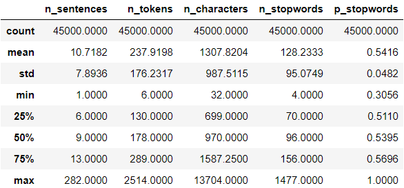

We have the answers to the first four questions in this table. Now, let’s see if it differs by sentiment. If they differ significantly, we could use the variable as a feature to the model:

我们有此表中前四个问题的答案。 现在，让我们看看它是否因情感而不同。 如果它们相差很大，我们可以将变量用作模型的功能：

num_vars = train.select_dtypes(np.number).columns
train.groupby("sentiment")[num_vars].agg(["mean", "median"])

From looking at central tendency, it doesn’t appear to differ by sentiment substantially. Just to be sure, let’s look at the distribution:

从集中趋势看，似乎没有实质性的差异。 可以肯定的是，让我们看一下分布：

# Create dataframe per sentiment
positives = train.query("sentiment=='positive'")
negatives = train.query("sentiment=='negative'")def plot_distribution(both, positives, negatives, var):
    """Plot overlayed histogram and density plot per sentiment."""
    fig, ax = plt.subplots(nrows=1, ncols=2, figsize=[16,4])
    # Histogram
    sns.distplot(negatives[var], bins=30, label="negative", kde=False, ax=ax[0], color='red')
    sns.distplot(positives[var], bins=30, label="positive", kde=False, ax=ax[0], color='green')
    ax[0].set_title(f"Histogram for {var}")
    ax[0].legend()
    # Density plot
    sns.kdeplot(negatives[var], label="negative", shade=True, ax=ax[1], color='red')
    sns.kdeplot(positives[var], label="positive", shade=True, ax=ax[1], color='green')
    ax[1].set_title(f"Density plot for {var}");
# Plot for all numerical variables
for var in num_vars:
    plot_distribution(train, positives, negatives, var)

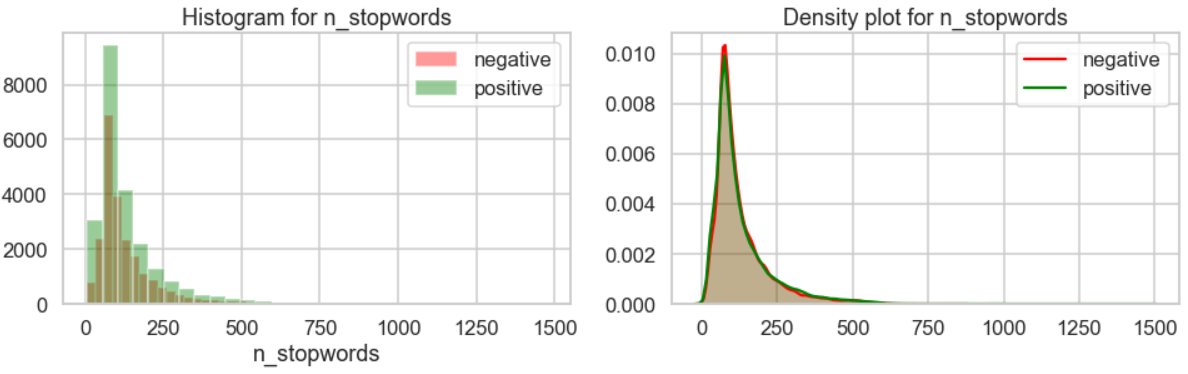
The distribution of variables seem pretty similar between sentiments. It’s unlikely that they will be useful as features, but we could always experiment. Maybe we could add this to a list of nice-to-try items?

情绪之间的变量分布似乎非常相似。 它们不太可能用作功能，但我们可以随时进行试验。 也许我们可以将其添加到试用项目列表中 ？

Before we wrap up, let’s look at one last thing - whether common words differ by sentiment. Let’s prepare the data for each sentiment:

在总结之前，让我们看看最后一件事-常用词是否因情感而异。 让我们为每个情绪准备数据：

def get_frequent_tokens(df_text, stop_words):
    # 1. Convert to one giant string
    string_text = " ".join(df_text.values)
    # 2. Tokenise to alphabetic tokens
    tokeniser = RegexpTokenizer("[A-Za-z]+")
    tokens = tokeniser.tokenize(string_text)
    # 3. Lowercase and lemmatise
    lemmatiser = WordNetLemmatizer()
    tokens = [lemmatiser.lemmatize(t.lower(), "v") for t in tokens]
    # 4. Remove stopwords
    tokens = [t for t in tokens if t not in stop_words]
    # 5. Prepare frequency distribution
    freq = FreqDist(tokens)
    return freq# Find frequent tokens by sentiment
pos_freq = get_frequent_tokens(positives['review'], stop_words)
neg_freq = get_frequent_tokens(negatives['review'], stop_words)# Create a union of top 20 tokens per sentiment
pos_common = [t for t, c in pos_freq.most_common(20)]
neg_common = [t for t, c in neg_freq.most_common(20)]
common = set(neg_common).union(pos_common)print(f"***** 20 frequent tokens in positive reviews: *****\n{pos_common}\n")
print(f"***** 20 frequent tokens in negative reviews: *****\n{neg_common}\n")
print(f"***** Their union: *****\n{common}\n")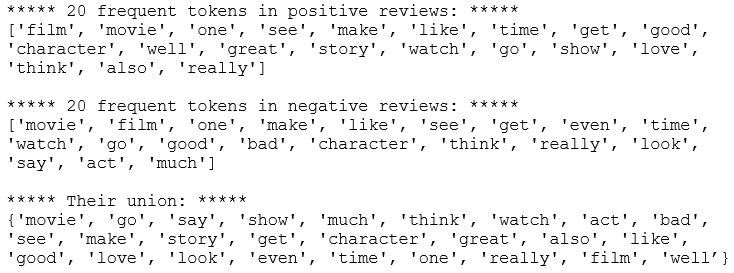

The 3 most common tokens in both sentiments are ‘film’, ‘movie’ and ‘one’. Let’s look at their frequencies:

两种情绪中最常见的3种标记是“电影”，“电影”和“一个”。 让我们看看它们的频率：

# Create a dataframe containing the common tokens and their frequency
common_freq = pd.DataFrame(index=common, columns=["neg", "pos"])
for token in common:
    common_freq.loc[token, "pos"] = pos_freq[token]
    common_freq.loc[token, "neg"] = neg_freq[token]
common_freq.sort_values(by="pos", inplace=True)# Add ranks and rank difference
common_freq['pos_rank'] = common_freq['pos'].rank()
common_freq['neg_rank'] = common_freq['neg'].rank()
common_freq['rank_diff'] = common_freq['neg_rank'] - common_freq['pos_rank']
common_freq.sort_values(by='rank_diff', inplace=True)
common_freq.head()

Now, time to visualise:

现在，是时候可视化了：

fig, ax =plt.subplots(1, 2, figsize=(16, 10))
sns.barplot(x="pos", y=common_freq.index, data = common_freq, ax=ax[0])
sns.barplot(x="neg", y=common_freq.index, data = common_freq, ax=ax[1])
fig.suptitle('Top tokens and their frequency by sentiment');

Hmm, it’s interesting to see ‘film’ is more frequent than ‘movie’ in positive reviews. In negative reviews, it’s flipped. Maybe they shouldn’t be added to stop words after all despite their frequency. Let’s look at the chart again, but excluding these two common words:

嗯，有趣的是，在正面评价中，“电影”比“电影”更常见。 在负面评论中，它被翻转了。 毕竟，尽管它们频繁出现，但不应该添加它们来停止单词。 让我们再次看一下图表，但排除以下两个常用词：

rest = common_freq.index.drop(['film', 'movie'])
fig, ax =plt.subplots(1, 2, figsize=(16, 10))
sns.barplot(x="pos", y=rest, data = common_freq.loc[rest], ax=ax[0])
sns.barplot(x="neg", y=rest, data = common_freq.loc[rest], ax=ax[1])
fig.suptitle('Top tokens and their frequency by sentiment');

It’s intuitive to see that the word ‘great’, ‘well’ and ‘love’ are more frequent in positive reviews whereas ‘even’ and ‘bad’ are more frequent in negative reviews.

从直观上可以看出，正面评价中的“伟大”，“好”和“爱”一词更为常见，而负面评价中的“偶数”和“不好”一词则更为常见。

There are still many things to explore, but it’s time to wrap up! 🕛

仍然有很多事情要探索，但是该总结了！ 🕛

3.结束语💭 (3. Final remarks 💭)

Well done to you for making this far! 😎 Let’s summarise the key points:◼️ Remove punctuation and numbers when tokenising◼️ Normalise text (lowercase, lemmatise, etc)◼️ Enrich stop words with ‘br’ and other missing auxillary verbs◼️ Remove rare words

到目前为止，您做得好！ 😎让我们总结关键点：◼️在标记化时删除标点符号和数字◼️规范化文本(小写，lemmatise等)◼️用'br'和其他缺失的辅助动词丰富停用词◼️删除稀有单词

A list of nice-to-try items: ◼️ Convert British spelling to American spelling (or vice versa)◼️ Keep numbers and convert them to words◼️ Keep hyphenated words as they are when tokenising◼️ Include bigrams◼️ Add numerical features such as number of sentences, tokens, characters and stop words

易于尝试的项目列表：◼️将英式拼写转换为美式拼写(反之亦然)◼️保留数字并将其转换为单词◼️保留带连字符的单词在进行标记化时保持原样big️包括双字母组◼️添加数字功能，例如数字句子，记号，字符和停用词

Thank you for reading my post. Exploratory data analysis is an open-ended and subjective task. You may have noticed that we had to make many small choices when exploring and preprocessing. Hopefully, this post gave you a taste of how to structure the analysis and showed example questions you could think about during the process. Having done some exploratory analysis, we are one step closer to building a model. In the next post, we will prepare the data for the model. Here are links to the other two posts of the series. *** (links to be added when published) ***◼️ Preprocessing text in Python◼️ Sentiment classifier in Python

感谢您阅读我的帖子。 探索性数据分析是一项开放性且主观的任务。 您可能已经注意到，在探索和预处理时，我们不得不做出许多小的选择。 希望这篇文章使您对如何构建分析有所了解，并展示了您在此过程中可以考虑的示例问题。 在进行了一些探索性分析之后，我们离建立模型又迈进了一步。 在下一篇文章中，我们将为模型准备数据。 这里是本系列其他两个帖子的链接。 ***(发布时添加链接)*** Python中的预处理文本Python Python中的情感分类器

Here are links to the my other NLP-related posts:◼️ Simple wordcloud in Python◼️️ Introduction to NLP — Part 1: Preprocessing text in Python◼️ Introduction to NLP — Part 2: Difference between lemmatisation and stemming◼️ Introduction to NLP — Part 3: TF-IDF explained◼️ Introduction to NLP — Part 4: Supervised text classification model in Python

以下是与我其他与NLP相关的文章的链接：◼️Python中的简单wordcloud◼️️NLP 简介—第1部分：Python中的预处理文本 ◼️NLP 简介—第2部分：lemmatisation和阻止词干之间的区别 ◼️NLP 简介—第3部分：TF-IDF解释了 ◼️NLP 简介—第4部分：Python中的监督文本分类模型

Bye for now 🏃💨

再见for

翻译自: https://towardsdatascience.com/exploratory-text-analysis-in-python-8cf42b758d9e

python 探索性分析