独家 | 文本数据探索性数据分析结合可视化和NLP产生见解（附代码）

作者：Susan Li

翻译：吴金笛

校对：和中华

本文约5000字，建议阅读12分钟。

本文使用电子商务的评价数据集作为实例来介绍基于文本数据特征的数据分析和可视化。

作为数据科学家或NLP专家，可视化地表示文本文档的内容是文本挖掘领域中最重要的任务之一。然而，在可视化非结构化 (文本)数据和结构化数据之间存在一些差距。

 

Photo credit: Pixabay

 

文本文档内容的可视化表示是文本挖掘领域中最重要的任务之一。作为一名数据科学家或NLP专家，我们不仅要从不同方面和不同细节层面来探索文档的内容，还要总结单个文档，显示单词和主题，检测事件，以及创建故事情节。

 

然而，在可视化非结构化(文本)数据和结构化数据之间存在一些差距。例如，许多文本可视化并不直接表示文本，而是表示语言模型的输出(字数、字符长度、单词序列等)。

 

在这篇文章中，我们将使用女装电子商务评论的数据集，并尝试使用Plotly的Python图形库和Bokeh可视化库尽可能多地探索和可视化。我们不仅将研究文本数据，而且还将可视化数值型和类别型特征。让我们开始吧!

 

数据

 

1. df = pd.read_csv('Womens Clothing E-Commerce Reviews.csv')  

 

表1

 

经过对数据的简单检查，发现我们需要进行一系列的数据预处理。

• 删除“Title”特征。

• 删除缺少“Review Text”的行。

• 清洗“Review Text”列。

• 使用TextBlob计算位于[-1,1]范围内的情绪极性，其中1表示积极情绪，-1表示消极情绪。

• 为评论的长度创建新特性。

• 为评论的字数创建新特性。

  
  

1. df.drop('Unnamed: 0', axis=1, inplace=True)  

2. df.drop('Title', axis=1, inplace=True)  

3. df = df[~df['Review Text'].isnull()]  

4.   

5. def preprocess(ReviewText):  

6.     ReviewText = ReviewText.str.replace("(  

7. )", "")  

8.     ReviewText = ReviewText.str.replace('().*()', '')  

9.     ReviewText = ReviewText.str.replace('(&)', '')  

10.     ReviewText = ReviewText.str.replace('(>)', '')  

11.     ReviewText = ReviewText.str.replace('(<)', '')  

12.     ReviewText = ReviewText.str.replace('(\xa0)', ' ')    

13.     return ReviewText  

14. df['Review Text'] = preprocess(df['Review Text'])  

15.   

16. df['polarity'] = df['Review Text'].map(lambda text: TextBlob(text).sentiment.polarity)  

17. df['review_len'] = df['Review Text'].astype(str).apply(len)  

18. df['word_count'] = df['Review Text'].apply(lambda x: len(str(x).split()))  

text_preprocessing.py

 

为了预览情绪极性分数是否有效，我们随机选择5个具有最高情绪极性分数（即1）的评论：

 

1. print('5 random reviews with the highest positive sentiment polarity: \n')  

2. cl = df.loc[df.polarity == 1, ['Review Text']].sample(5).values  

3. for c in cl:  

4.     print(c[0])  

 

图1

 

然后随机选择5个具有最中性情绪级性的评论（即0）：

1. print('5 random reviews with the most neutral sentiment(zero) polarity: \n')  

2. cl = df.loc[df.polarity == 0, ['Review Text']].sample(5).values  

3. for c in cl:  

4.     print(c[0])  

 

图2

 

只有2个评论有最负面的情绪级性分：

1. print('2 reviews with the most negative polarity: \n')  

2. cl = df.loc[df.polarity == -0.97500000000000009, ['Review Text']].sample(2).values  

3. for c in cl:  

4.     print(c[0])  

 

图3

 

有效！

 

使用Plotly进行单变量可视化

 

单变量可视化是最简单的可视化类型，其仅包括对单个特征或属性的观察。 单变量可视化包括直方图，条形图和折线图。

 

商品评论情绪极性分数的分布

1. df['polarity'].iplot(  

2.     kind='hist',  

3.     bins=50,  

4.     xTitle='polarity',  

5.     linecolor='black',  

6.     yTitle='count',  

7.     title='Sentiment Polarity Distribution')  

图4

 

绝大多数情绪极性分数大于零，意味着大多数情绪非常积极。

 

评论等级的分布

1. df['Rating'].iplot(  

2.     kind='hist',  

3.     xTitle='rating',  

4.     linecolor='black',  

5.     yTitle='count',  

6.     title='Review Rating Distribution')  

 

图5

 

等级与极性分数一致，即大多数等级都相当高，都是4或5。

 

评论者的年龄分布

1. df['Age'].iplot(  

2.     kind='hist',  

3.     bins=50,  

4.     xTitle='age',  

5.     linecolor='black',  

6.     yTitle='count',  

7.     title='Reviewers Age Distribution')  

 

图6

 

大多数评论者都在30到50岁之间。

 

评论文本长度的分布

1. df['review_len'].iplot(  

2.     kind='hist',  

3.     bins=100,  

4.     xTitle='review length',  

5.     linecolor='black',  

6.     yTitle='count',  

7.     title='Review Text Length Distribution')  

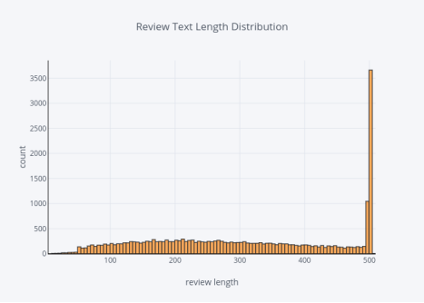
图7

 

评论单词数的分布

1. df['word_count'].iplot(  

2.     kind='hist',  

3.     bins=100,  

4.     xTitle='word count',  

5.     linecolor='black',  

6.     yTitle='count',  

7.     title='Review Text Word Count Distribution')  

图8

 

有很多人喜欢留下长篇评论。

对于类别型特征，我们只需使用条形图来显示频率。

 

division的分布

1.df.groupby('DivisionName').count(['Clothing ID'].iplot(kind='bar', yTitle='Count', linecolor='black', opacity=0.8, title='Bar chart of Division Name', xTitle='Division Name')  

 

图9

 

General Division的评论数量最多，而Initmates division的评论数量最少。

 

部门的分布

1.df.groupby('DepartmentName').count(['Clothing ID'].sort_values(ascending=False).iplot(kind='bar', yTitle='Count', linecolor='black', opacity=0.8, title='Bar chart of Department Name', xTitle='Department Name')  

图10

 

当讨论部门时，Tops部门的评论最多，Trend部门的评论数量最少。

 

类别的分布

1..groupby('Classame').count(['Clothing ID'].sort_values(ascending=False).iplot(kind='bar', yTitle='Count', linecolor='black', opacity=0.8, title='Bar chart of Class Name&#