使用python进行数据分析和机器学习的实用指南

A hands-on guide to mastering the first baby steps in building Machine Learning applications.

在构建机器学习应用程序方面掌握入门的第一步的动手指南。

Machine Learning is continuously evolving. Along with that evolution comes a spike in demand and importance. Corporations and startups are needing Data Scientists and Machine Learning Engineers now more than ever to turn those troves of data into useful wisdom. There’s probably not a better time than now (except 5 years ago) to delve into Machine Learning. And of course, there’s not a better tool to develop those applications than Python. Python has a vibrant and active community. Many of its developers came from the scientific community, thus providing Python with vast numbers of libraries for scientific computing.

机器学习在不断发展。 随之而来的是需求和重要性的激增。 公司和初创企业现在比以往任何时候都更需要数据科学家和机器学习工程师，以将这些数据变成有用的智慧。 探究机器学习的时间可能比现在(5年前除外)要好。 当然，没有比Python更好的工具来开发这些应用程序。 Python具有活跃而活跃的社区。 它的许多开发人员都来自科学界，因此为Python提供了大量用于科学计算的库。

In this article, we will discuss some of the features of Python’s key scientific libraries and also employ them in a proper Data Analysis and Machine Learning workflow.

在本文中，我们将讨论Python关键科学库的某些功能，并在适当的数据分析和机器学习工作流程中使用它们。

What you will learn;

您将学到什么；

• Understand what Pandas is and why it is very integral to your workflow.
  了解什么是熊猫，以及为什么它对您的工作流程非常重要。
• How to use Pandas to inspect your dataset
  如何使用熊猫检查数据集
• How to prepare the data and feature-engineer with Pandas
  如何使用Pandas准备数据和功能工程师
• Understand why Data Visualization matters.
  了解为什么数据可视化很重要。
• How to visualize data with Matplotlib and Seaborn.
  如何使用Matplotlib和Seaborn可视化数据。
• How to build a statistical model with Statsmodel.
  如何使用Statsmodel建立统计模型。
• How to build an ML model with Scikit-Learn’s algorithms.
  如何使用Scikit-Learn的算法构建ML模型。
• How to rank your model’s feature importances and perform feature selection.
  如何对模型的特征重要性进行排名并执行特征选择。

If you’d like to go straight to code, it is here on GitHub.

如果您想直接编写代码，请访问GitHub上的代码。

Disclaimer: This article assumes that

免责声明：本文假设

• You have at least, a usable knowledge of Python and
  您至少具有Python的可用知识，并且

• You already are familiar with the Data Science/Machine Learning workflow.

  您已经熟悉了数据科学/机器学习工作流程 。

大熊猫 (Pandas)

Pandas is an extraordinary tool for data analysis built to become the most powerful and flexible open-source data analysis/manipulation tool available in any language. Let’s take a look at what Pandas is capable of:

Pandas是用于数据分析的非凡工具，旨在成为任何语言中功能最强大，最灵活的开源数据分析/操纵工具。 让我们看一下熊猫的功能：

数据采集 (Data Acquisition)

import numpy as np
import pandas as pd
from sklearn import datasetsiris_data = datasets.load_iris()iris_data.keys()# THIS IS THE OUTPUT FOR 'iris_data.keys()'
dict_keys(['data', 'target', 'frame', 'target_names', 'DESCR', 'feature_names', 'filename'])iris_data['target_names']# THIS IS THE OUTPUT FOR 'iris_data['target_names']'
array(['setosa', 'versicolor', 'virginica'], dtype='<U10')df_data = pd.DataFrame(iris_data['data'], columns=iris_data['feature_names'])df_target = pd.DataFrame(iris_data['target'], columns=['species'])df = pd.concat([df_data, df_target], axis=1)df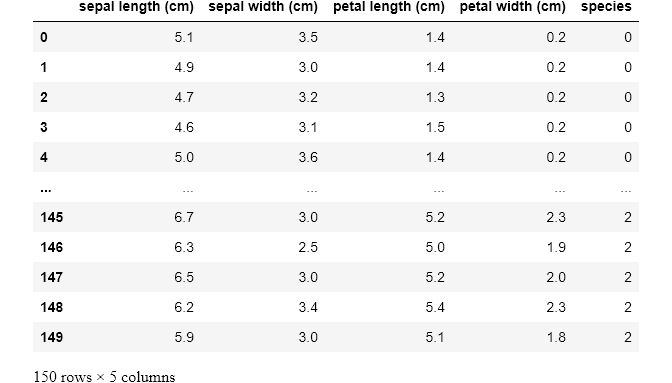

In the above cells, you’d notice that I have imported the classic dataset, the Iris dataset, using Scikit-learn (we’ll explore Scikit-learn later on). I then passed the data into a Pandas DataFrame while also including the column headers. I also created another DataFrame to contain the iris species which were code-named 0 for setosa, 1 for versicolor, and 2 for virginica. The final step was to concatenate the two DataFrames into a single DataFrame.

在上面的单元格中，您会注意到我已经使用Scikit-learn导入了经典数据集Iris数据集 (稍后我们将探讨Scikit-learn)。 然后，我将数据传递到Pandas DataFrame中，同时还包括列标题。 我还创建了另一个DataFrame来包含虹膜种类，这些虹膜种类分别是setosa 0 ， versicolor 1和virginica 2 。 最后一步是将两个DataFrame串联为一个DataFrame。

When working with data that can fit on a single machine, Pandas is the ultimate tool. It’s more like Excel but on steroids. Just like Excel, the basic units of operations are rows and columns where columns of data are Series, and a collection of Series is the DataFrame.

当处理可放在单个计算机上的数据时，Pandas是终极工具。 它更像Excel，但在类固醇上。 与Excel一样，基本的操作单位是行和列，其中数据列是Series，而Series的集合是DataFrame。

探索性数据分析 (Exploratory Data Analysis)

Let’s perform a few common operations;

让我们执行一些常见的操作；

数据切片 (Data Slicing)

df.head()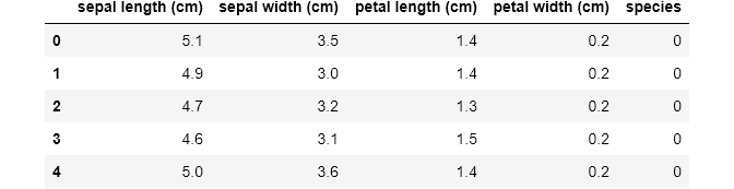

df['sepal length (cm)']# OUTPUT
0      5.1
1      4.9
2      4.7
3      4.6
4      5.0
      ... 
145    6.7
146    6.3
147    6.5
148    6.2
149    5.9
Name: sepal length (cm), Length: 150, dtype: float64

The .head() command will return the first 5 rows. The second command was to select a single column from the DataFrame by referencing it with the column name.

.head()命令将返回前5行。 第二个命令是通过使用列名称引用它来从DataFrame中选择单个列。

A different way of performing data slicing is by using the loc and iloc methods.

执行数据切片的另一种方法是使用loc和iloc方法。

To use iloc, we have to specify the rows and columns we want to slice by their integer index, while for loc, we have to specify the names of the columns that we want to filter out.

要使用iloc ，我们必须通过整数索引指定要切片的行和列，而对于loc ，我们必须指定要过滤出的列的名称。

loc gets row (or columns) with a particular label from the index while iloc gets rows (or columns) location at particular positions in the index (so it only takes integers)

loc从索引中获取具有特定标签的行(或列) ，而iloc获取索引中特定位置的行(或列)位置(因此仅获取整数)

df.iloc[:3, :2]

Using .iloc, we just selected the first 3 rows and 2 columns of the DataFrame. Let’s try something more difficult;

使用.iloc ，我们只选择了.iloc的前3行和2列。 让我们尝试一些更困难的事情；

df.loc[:3, [x for x in df.columns if 'width' in x]]

Here we iterate through df.columns, which would return a list of columns, and select only the columns with “width” in their names. This seemingly small function is quite a powerful tool when employed on far larger datasets.

在这里，我们遍历df.columns ，它将返回列列表，并仅选择名称中带有“ width”的列。 当在大得多的数据集上使用时，这个看似很小的函数是一个非常强大的工具。

Next, let’s use another way of selecting a portion of the data by specifying a condition to be satisfied. We’ll look at the unique list of species, then select one of those.

接下来，让我们使用另一种方法，通过指定要满足的条件来选择部分数据。 我们将查看唯一的species列表，然后选择其中一个。

# Listing all the available unique classesdf['species'].unique()# OUTPUT FOR 'df['species'].unique()'
array([0, 1, 2])df[df['species'] == 2]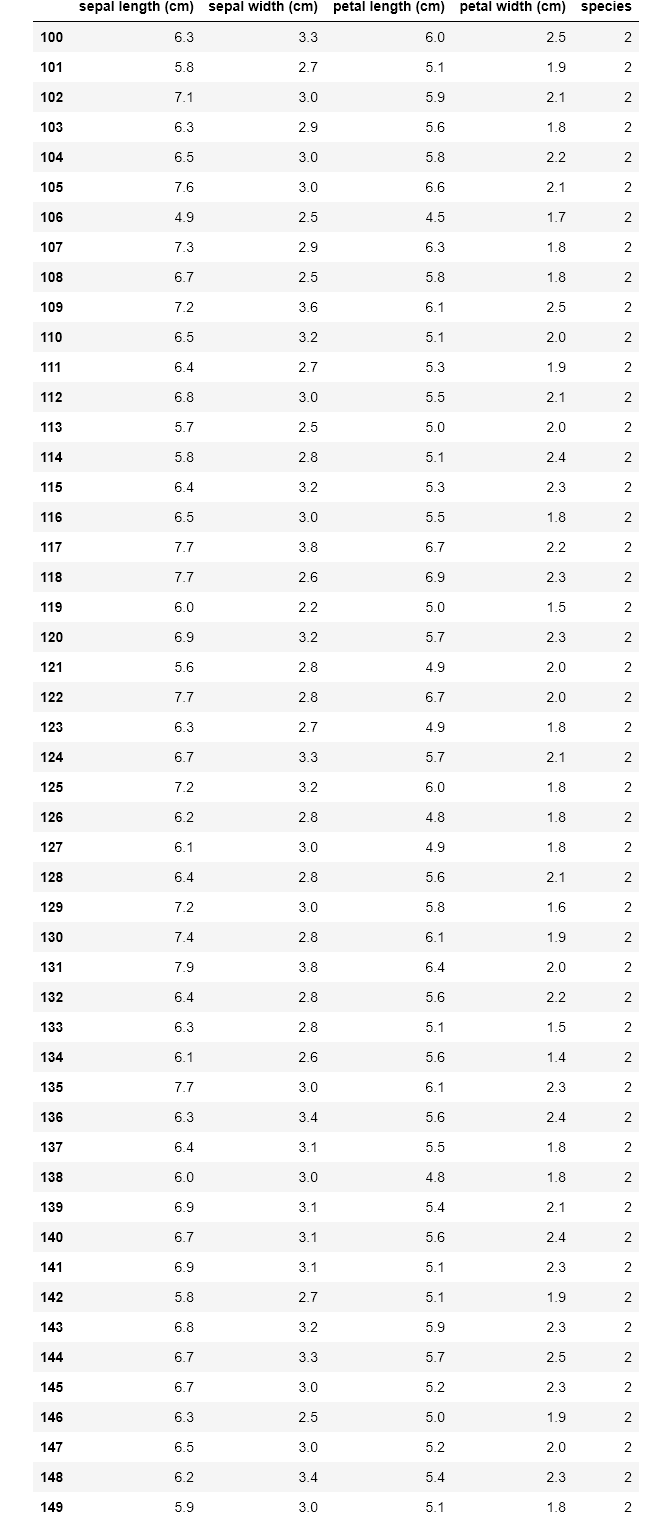

Notice that our DataFrame only contains rows of Iris-virginica species (represented by 2). In fact, the size is 50, as opposed to the original 150 rows.

请注意，我们的DataFrame仅包含Iris-virginica属弗吉尼亚种的行(以2表示)。 实际上，大小为50，而不是原始的150行。

df.count()# OUTPUT
sepal length (cm)    150
sepal width (cm)     150
petal length (cm)    150
petal width (cm)     150
species              150
dtype: int64df[df['species'] == 2].count()# OUTPUT
sepal length (cm)    50
sepal width (cm)     50
petal length (cm)    50
petal width (cm)     50
species              50
dtype: int64

You’d also notice that the index on the left retains the original row numbers, which might cause issues later. So we could save it as a new DataFrame and reset the index.

您还会注意到，左侧的索引保留了原始行号，以后可能会引起问题。 因此，我们可以将其另存为新的DataFrame并重置索引。

virginica = df[df['species'] == 2].reset_index(drop=True)
virginica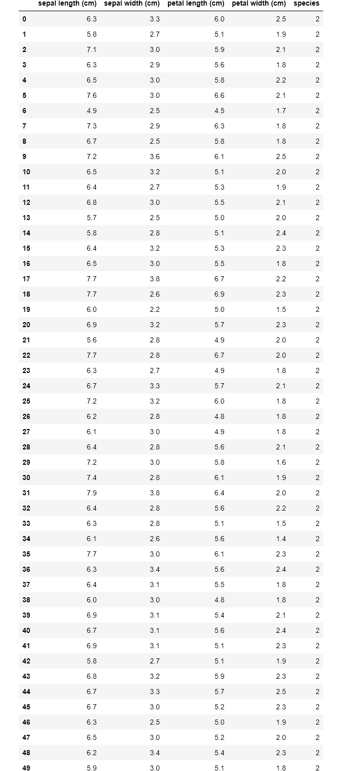

We selected this new DataFrame by specifying a condition. Now let’s add more conditions. We’ll specify two conditions on our original DataFrame.

我们通过指定条件选择了这个新的DataFrame。 现在让我们添加更多条件。 我们将在原始DataFrame上指定两个条件。

df[(df['species'] == 2) & (df['petal width (cm)'] > 2.2)]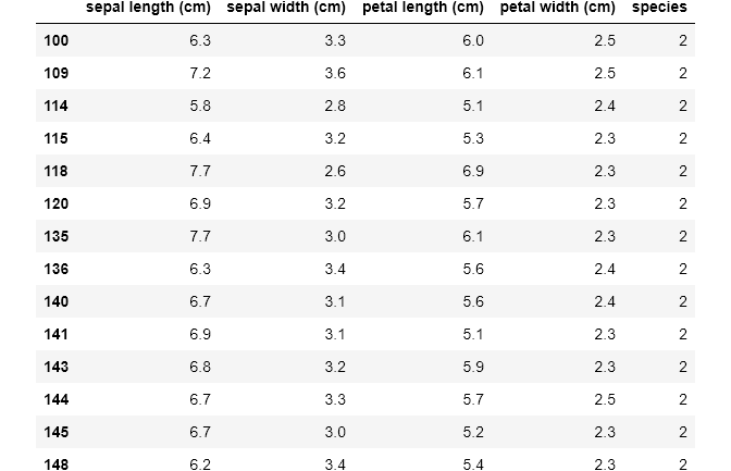

You may reset the index of this new DataFrame by yourself, as an exercise.

作为练习，您可以自己重置此新DataFrame的索引。

描述性统计 (Descriptive Statistics)

Now let’s try and get some descriptive statistics from our dataset;

现在，让我们尝试从数据集中获取一些描述性统计信息；

df.describe()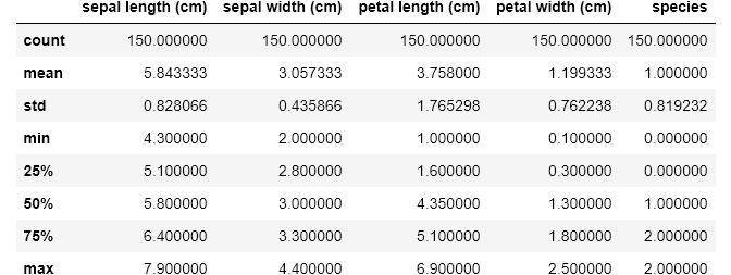

Using .describe() method, I just received a breakdown of the descriptive statistics for each of the columns. I could spot the counts of all the columns and easily note if there are missing values. I could see the mean, standard deviation, median, mode, and I could also note if the data is skewed. I could also pass in my own percentiles if I want more granular information;

使用.describe()方法，我刚刚收到了每一列的描述性统计数据的细分。 我可以发现所有列的计数，并轻松记录是否有缺失值。 我可以看到平均值，标准偏差，中位数，众数，也可以注意到数据是否倾斜。 如果我想获得更详细的信息，我也可以传递自己的百分位数。

# Passing in custom percentilesdf.describe(percentiles=[.2, .4, .8, .9, .95])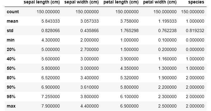

Now let’s check if there is any correlation between the features by calling .corr() method on the DataFrame;

现在，通过在DataFrame上调用.corr()方法来检查功能之间是否存在任何关联。

# Checking for correlations between the featuresdf.corr()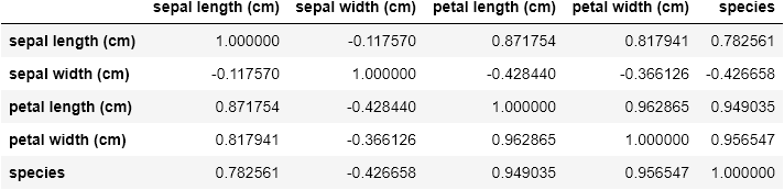

I find it surprising that sepal length and sepal width has the lowest correlation with a score of -0.117570.

我感到惊讶的是， sepal length和sepal width具有最低的相关性，得分为-0.117570 。

Now that we’ve understood how to select subsets of our DataFrame and how to summarize its statistics, let’s try and visually inspect our data.

现在，我们已经了解了如何选择DataFrame的子集以及如何汇总其统计信息，让我们尝试并直观地检查我们的数据。

数据可视化 (Data Visualization)

You might wonder why we should even bother with visualization. The fact is that Data Visualization makes data easier for the human brain to understand and we can easily detect trends, patterns, and outliers in our data by performing a visual inspection.

您可能想知道为什么我们还要打扰可视化。 事实是，数据可视化使人脑更容易理解数据，并且我们可以通过执行视觉检查来轻松检测数据中的趋势，模式和异常值。

So now that we understand the importance of visualization, let’s take a look at a pair of Python libraries that do this best.

因此，既然我们了解了可视化的重要性，那么让我们看一下最能做到这一点的一对Python库。

Matplotlib库 (The Matplotlib Library)

Matplotlib is the great grandfather of all Python plotting libraries. It was originally created to emulate the plotting functionality of MATLAB, and it grew into a giant in its own right.

Matplotlib是所有Python绘图库的曾祖父。 它最初是为了模拟MATLAB的绘图功能而创建的，它本身就发展成为一个巨大的公司。

import matplotlib.pyplot as plt
plt.style.use('ggplot')

The first line imports Matplotlib while the 2nd line sets our plotting style to resemble R’s ggplot library.

第一行导入Matplotlib，第二行将我们的绘图样式设置为类似于R的ggplot库 。

Now let’s generate our first graph with the following code on our regular dataset;

现在，让我们在常规数据集中使用以下代码生成第一个图；

# Plotting an histogram of the petal width featureplt.figure(figsize=(6,4))
plt.hist(df['petal width (cm)'], color='black')
plt.xlabel('Width', fontsize=12)
plt.ylabel('Count', fontsize=12)
plt.title('Iris Petal Width', fontsize=14,)Text(0.5, 1.0, 'Iris Petal Width')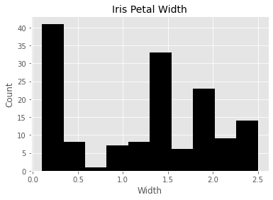

Let’s go through the code line by line:

让我们逐行浏览代码：

• The first line creates a plotting space with a width of 6 inches and a height of 4 inches.
  第一行创建一个绘图空间，其宽度为6英寸，高度为4英寸。
• The second line creates a histogram of the petal width column and we also set the bar color to black.
  第二行创建花瓣宽度列的直方图，我们还将条形颜色设置为黑色。
• We labeled the x and y axes with “Width” and “Count” respectively while also setting the font size to 12.
  我们分别将x轴和y轴标记为“宽度”和“计数”，同时还将字体大小设置为12。
• The final line creates the title “Iris Petal Width” with a font size of 14.
  最后一行创建标题“虹膜花瓣宽度”，字体大小为14。

All these together gives us a nicely labeled histogram of our petal width data!

所有这些共同为我们提供了花瓣宽度数据的标签直方图！

Let’s now expand on that and generate histograms for each column of our Iris dataset;

现在让我们对其进行扩展，并为Iris数据集的每一列生成直方图。

# Plotting subplots of the 4 features (NOTE: THIS IS NOT IDEAL!)fig, ax = plt.subplots(2, 2, figsize=(6,4))ax[0][0].hist(df['petal width (cm)'], color='black')
ax[0][0].set_xlabel('Width', fontsize=12)
ax[0][0].set_ylabel('Count', fontsize=12)
ax[0][0].set_title("Iris Petal Width", fontsize=14)ax[0][1].hist(df['petal length (cm)'], color='black')
ax[0][1].set_xlabel('Length', fontsize=12)
ax[0][1].set_ylabel('Count', fontsize=12)
ax[0][1].set_title("Iris Petal Length", fontsize=14)ax[1][0].hist(df['sepal width (cm)'], color='black')
ax[1][0].set_xlabel('Width', fontsize=12)
ax[1][0].set_ylabel('Count', fontsize=12)
ax[1][0].set_title("Iris Sepal Width", fontsize=14)ax[1][1].hist(df['sepal length (cm)'], color='black')
ax[1][1].set_xlabel('Length', fontsize=12)
ax[1][1].set_ylabel('Count', fontsize=12)
ax[1][1].set_title("Iris Sepal Length", fontsize=14)plt.tight_layout()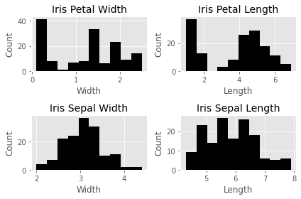

This is not the most efficient way to do this, obviously, but it is quite useful to demonstrate how Matplotlib works. With the previous example, this is almost self-explanatory except that we now have four subplots that can be accessed through the ax array. Another addition is the plt.tight_layout() call, which we nicely auto-space our subplots to avoid crowding.

显然，这不是最有效的方法，但是它对演示Matplotlib的工作原理非常有用。 在前面的示例中，这几乎是不言而喻的，除了我们现在可以通过ax数组访问四个子图。 另一个添加是plt.tight_layout()调用，我们很好地自动plt.tight_layout()了子图以避免拥挤。

Let’s now take a look at the other kinds of plots available in Matplotlib. One is scatterplot. Here we plot the petal width against the petal length;

现在让我们看一下Matplotlib中可用的其他类型的图。 一种是散点图 。 在这里，我们针对花瓣长度绘制花瓣宽度；

# A scatterplot of the Petal Width against the Petal Lengthplt.scatter(df['petal width (cm)'], df['petal length (cm)'], color='green')
plt.xlabel('Petal Width')
plt.ylabel('Petal Length')
plt.title('Petal Scatterplot')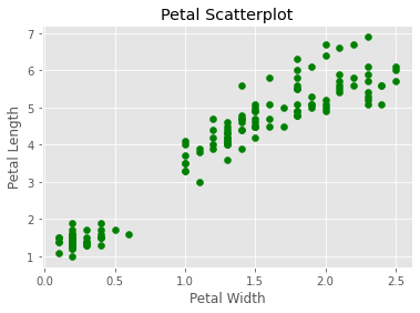

Another plot is a simple line plot. Here is a line plot of the petal length;

另一个图是简单的线图。 这是花瓣长度的线图；

# A simple line plot of the Petal Lengthplt.figure(figsize=(6,6))
plt.plot(df['petal length (cm)'], color='blue')
plt.xlabel('Specimen Number')
plt.ylabel('Petal Length')
plt.title('Petal Length Plot')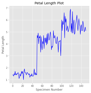

We can see here that there are three distinct clusters in this plot, presumably for each kind of species. This tells us that the petal length would most likely be a useful feature to denote the species if we build a classifier model.

我们可以在这里看到该图中有三个不同的簇，大概是每种物种的簇。 这告诉我们，如果我们建立分类器模型，则花瓣长度很可能是表示物种的有用功能。

Finally, let’s look at the bar chart. Here we’ll plot a bar chart for the mean of each feature for the three species of irises. Also, we will make it a stacked bar chart, to spice things up.

最后，让我们看一下条形图。 在这里，我们将为三种虹膜的每个特征的平均值绘制条形图。 另外，我们将它做成堆积的条形图，以使事情变得有趣。

# A Bar-chart of the mean of each feature for the 3 classes of irisesfig, ax = plt.subplots(figsize=(6,6))
labels = [x for x in df.columns if 'length' in x or 'width' in x]ver_y = [df[df['species'] == 0][x].mean() for x in labels]
vir_y = [df[df['species'] == 1][x].mean() for x in labels]
set_y = [df[df['species'] == 2][x].mean() for x in labels]
x = np.arange(len(labels))plt.bar(x, vir_y, bottom=set_y, color='darkgrey')
plt.bar(x, set_y, bottom=ver_y, color='white')
plt.bar(x, ver_y, color='black')plt.xticks(x)
ax.set_xticklabels(labels, rotation=-70, fontsize=12);
plt.title('Mean Measurement by Class')
plt.legend(['Setosa', 'Versicolor', 'Virginica'])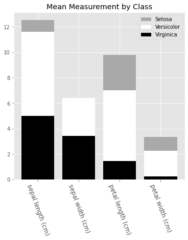

To generate a bar chart, we need to pass in the x and y values into .bar(). Here, the x values is an array of the length of the features that we are interested in. We also called the .setxtickslabels() and passed in our preferred column names for display.

要生成条形图，我们需要将x和y值传递给.bar() 。 在这里，x值是我们感兴趣的特征的长度的数组。我们还调用了.setxtickslabels()并传入了我们首选的列名以进行显示。

To line up the x labels properly, we also adjusted the spacing of the labels. This is why we set the xticks to x plus half the size of the bar_width.

为了正确对齐x标签，我们还调整了标签间距。 这就是为什么我们将xticks设置为x加bar_width大小的一半的原因。

The y values come from taking the mean of each feature for each species, and we called each by calling .bar(). We also pass in a bottom parameter for each series, to set the minimum y point and the maximum y point of the series below it. This is what creates the stacked bars.

y值来自每个物种的每个特征的均值，我们通过调用.bar()来调用每个y。 我们还为每个系列传递一个bottom参数，以在其下方设置系列的最小y点和最大y点。 这就是创建堆叠条形的原因。

And finally, we add a legend, which describes each series. The names are inserted into the legend list in order of the placement of the bars from top to bottom.

最后，我们添加一个图例，描述每个系列。 这些名称将按照从上到下的排列顺序插入到图例列表中。

西雅图图书馆 (The Seaborn Library)

The next visualization library we’ll have a look at is Seaborn. Seaborn is built on Matplotlib, and it is built for statistical visualizations. This means that it is tailor-made for structured data (data in rows and columns).

我们将要看的下一个可视化库是Seaborn。 Seaborn基于Matplotlib构建，并且为统计可视化而构建。 这意味着它是针对结构化数据(行和列中的数据)量身定制的。

Now let’s have a taste of the power of Seaborn. With just two lines of code, we’d get the following;

现在，让我们来品尝一下Seaborn的强大功能。 仅需两行代码，我们将获得以下内容：

import seaborn as snssns.pairplot(df, hue='species')<seaborn.axisgrid.PairGrid at 0x28fe2953430>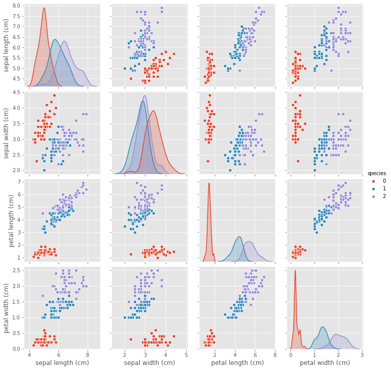

Having just gone through (what I hope it’s not) a torrid time understanding the intricacies of Matplotlib, you’d appreciate the simplicity and ease with which we generated this plot. All of our features were created and properly labeled with just two lines of code.

刚刚经历了(我希望不是)辛苦的时间，了解了Matplotlib的复杂性，您将欣赏我们生成此图的简便性。 我们所有的功能均已创建，并仅用两行代码正确标记。

You’d probably wonder why you’d want to use Matplotlib when Seaborn is so effortless to use. As I said earlier, Seaborn is built on Matplotlib, and you’d have to combine the functions of Seaborn with that of Matplotlib at times for modification. Let’s try out this next visualization;

您可能想知道为什么在Seaborn如此轻松地使用时为什么要使用Matplotlib。 正如我之前说的，Seaborn是基于Matplotlib构建的，您必须有时将Seaborn的功能与Matplotlib的功能结合起来进行修改。 让我们尝试下一个可视化；

sns.set(style='white', palette='muted')
features = [col for col in df.columns if '(cm)' in col]plt.figure(figsize=(7, 7))
for n in range(len(features)):
    plt.subplot(2, 2, n+1)
    sns.violinplot(x='species', y=features[n], data=df)
plt.suptitle('Violin Plots', fontsize=16)
plt.tight_layout()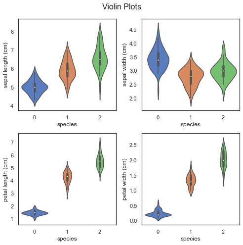

We have generated a violin plot for each of the four features. A violin plot displays the distribution of the features. For example, you can easily see that the petal length of setosa (0) is highly clustered between 1 cm and 2 cm, while virginica (2) is much more dispersed, from nearly 4 cm to over 7 cm.

我们为这四个功能中的每个功能生成了一个小提琴图。 小提琴图显示了特征的分布。 例如，您可以轻松地看到setosa (0)的花瓣高度集中在1 cm和2 cm之间，而virginica (2)的分散程度更强，从近4 cm到7 cm以上。

You will also notice that we have used much of the same code we used when constructing the matplotlib graphs. The main difference is the addition of the sns.plot() calls, in lieu of the previous plt.plot() and ax.plot() calls.

您还将注意到，在构造matplotlib图时，我们使用了许多相同的代码。 主要区别是增加了sns.plot()调用，以代替先前的plt.plot()和ax.plot()调用。

There is a wide range of graphs that you can create with Seaborn and Matplotlib, and I’d highly recommend delving into the documentation for these two libraries.

您可以使用Seaborn和Matplotlib创建大量图形，我强烈建议您深入研究这两个库的文档。

The ones we’ve discussed here should go a long way in helping you visualize and understand your subsequent data.

我们在这里讨论的内容在帮助您可视化和理解后续数据方面应该大有帮助。

资料准备 (Data Preparation)

Having understood how to inspect and visualize our data, the next step is to learn how to process and manipulate our data. And here, we’d be working with map(), apply(), applymap(), and groupby() functions of Pandas. They are invaluable in working with Data, and they are very useful for feature engineering, which is the art of creating new features.

了解了如何检查和可视化我们的数据之后，下一步就是学习如何处理和操纵我们的数据。 在这里，我们将使用applymap() map() ， apply() ， applymap()和groupby()函数。 它们在处理数据方面非常宝贵，并且对于要素工程(这是创建新要素的艺术)非常有用。

地图 (map)

The map function works only on series, so we'll use it to transform a column of our DataFrame, which is a Pandas series. Suppose we decide that we're tired of using the species code numbers? We can use map with a Python dictionary to achieve this. The keys will be the code numbers while the values will be the replacements

map函数仅适用于序列，因此我们将使用它来转换DataFrame的列，该列是Pandas系列。 假设我们认为我们已经厌倦了使用物种代码号吗？ 我们可以将map与Python字典结合使用来实现此目的。 键将是代码号，而值将是替换项

# Replacing each of the unique Iris typesdict_map = {0: 'SET', 
            1: 'VIR', 
            2: 'VER'}
df['species'] = df['species'].map(dict_map)
df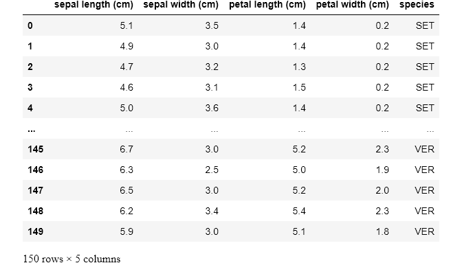

Here we have passed in our dictionary and the map function ran through our entire data, changing the code numbers to their replacements everywhere it encounters them.

在这里，我们传递了字典，并且map函数遍历了整个数据，将代码号更改为它们遇到的任何地方的替换项。

Had we chosen another name for our column, say better names, we'd have had a new column called better names appended to our DataFrame, and we'd still have the species column with the new better names column.

如果我们为列选择了另一个名称，例如“ better names ，我们将在DataFrame上追加一个名为“ better names的新列，并且仍然在“ species列中添加新的“ better names列。

We could also pass a series or a function into our map function, but we can also do this using the apply function (as we'd see soon). What sets the map function apart is the ability to pass in a Dictionary, hence making map the go-to function for most single-column transformation.

我们也可以将一个序列或一个函数传递到map函数中，但是我们也可以使用apply函数来做到这一点(很快就会看到)。 使map函数与众不同的是传递Dictionary的能力，因此使map成为大多数单列转换的首选函数。

应用 (apply)

Unlike map, apply works on both series (single columns) and DataFrames (collections of series). Now let's create a new column based on Petal width using the Petal width's mean (1.3) as the deciding factor.

与map不同，在序列(单列)和DataFrames(序列的集合)上都apply 。 现在，我们以“花瓣宽度”为基础创建一个新列，使用“花瓣宽度”的均值(1.3)作为决定因素。

If the petal width is greater than the mean, we'd set wide petal to 1, while if it is lower than the mean, we'd set wide petal to 0.

如果petal width是大于平均值，我们会设置wide petal为1，而如果它是低于平均值的，我们会设置wide petal为0。

# Creating a new feature via petal widthdf['wide petal'] = df['petal width (cm)'].apply(lambda x: 1 if x>=1.3 else 0)
df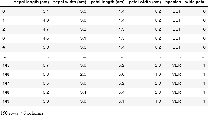

Here, we ran apply on the petal width column that returned the corresponding values in the wide petal column. The apply function works by running through each value of the petal width column. If the value is greater than or equal to 1.3, the function returns 1, otherwise it returns 0.

在这里，我们跑了apply上的petal width ，在返回的相应值的列wide petal列。 apply函数通过遍历“ petal width列的每个值来工作。 如果该值大于或等于1.3，则该函数返回1，否则返回0。

This type of transformation is a fairly common Feature Engineering technique in Machine Learning, so it is good to be familiar with how to perform it.

这种类型的转换是机器学习中相当普遍的特征工程技术，因此最好熟悉如何进行转换。

Now, let’s look at how to use apply across a DataFrame, and not just on a single Series. We’ll create a new column based on the petal area.

现在，让我们看看如何在整个DataFrame上使用Apply，而不仅仅是在单个Series上。 我们将基于花瓣区域创建一个新列。

# creating a new column via petal length & petal widthdf['petal area'] = df.apply(lambda row: row['petal width (cm)'] * row['petal length (cm)'], axis=1)
df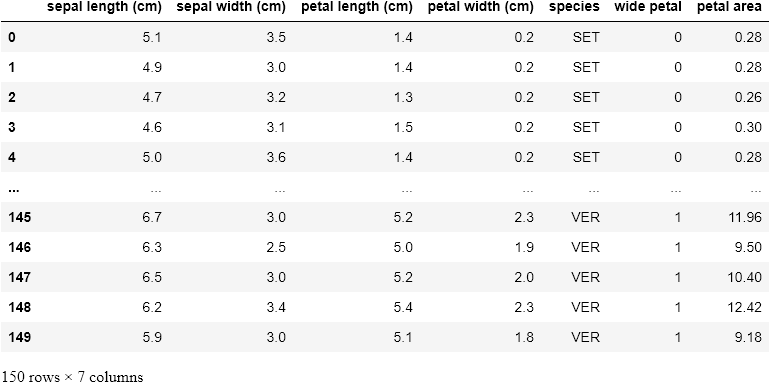

Notice that we called apply on the whole DataFrame here, and we also pass in a new argument, axis=1, so as to select the columns sequentially and apply the function row-wise. Had we set axis to 0, then the function would operate column-wise and throw up an error.

请注意，这里我们在整个DataFrame上调用了apply ，并且还传入了新参数axis=1 ，以便顺序选择列并逐行应用函数。 如果将axis设置为0，则该函数将按列进行操作并引发错误。

So for every row in the DataFrame, we multiply its petal width with its petal length, hereby creating a resultant series, wide petal.

因此，对于DataFrame中的每一行，我们将其petal width乘以其petal length ，从而创建一个结果序列，即wide petal 。

This kind of power and flexibility is what makes Pandas an indispensable tool for Data Manipulation.

这种强大的功能和灵活性使Pandas成为数据处理必不可少的工具。

套用地图 (applymap)

The applymap function is the tool to use when we want to manipulate all the data cells in a DataFrame. Let's take a look at this;

applymap函数是我们要操纵DataFrame中所有数据单元格时要使用的工具。 让我们看看这个；

# Getting the log values of all the data cellsdf.applymap(lambda x: np.log(x) if isinstance(x, float) else x)

Here we performed a log transformation (using Numpy) on the entire data and the condition stated is that the data cell must belong to a float instance.

在这里，我们对整个数据执行了日志转换(使用Numpy)，声明的条件是数据单元必须属于浮点型实例。

Common applications of applymap include transforming or formatting each cell based on meeting a number of conditions.

applymap常见应用包括基于满足许多条件来转换或格式化每个单元格。

通过...分组 (groupby)

And now, let’s have a look at an incredibly useful tool, but one that new Pandas users struggle to wrap their heads around. We’ll examine a number of examples in order to illustrate its common functionalities.

现在，让我们看一下一个非常有用的工具，但是新的Pandas用户却很难缠住它。 我们将研究许多示例，以说明其常见功能。

The groupby function does exactly what it is named: it groups data based on a class or some classes you choose. Let's try out the first example;

groupby函数的功能与它的名称完全相同：它根据您选择的一个或多个类对数据进行分组。 让我们尝试第一个例子；

df.groupby('species').mean()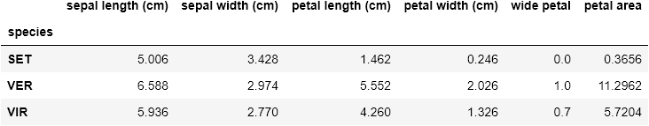

Here, data for each species is partitioned and the mean for each feature is provided. Now let’s take a larger step and get descriptive statistics for each species;

在此，将每个物种的数据进行分区，并提供每个特征的平均值。 现在让我们迈出更大的一步，获取每个物种的描述性统计数据；

# T for transposedf.groupby('species').describe().T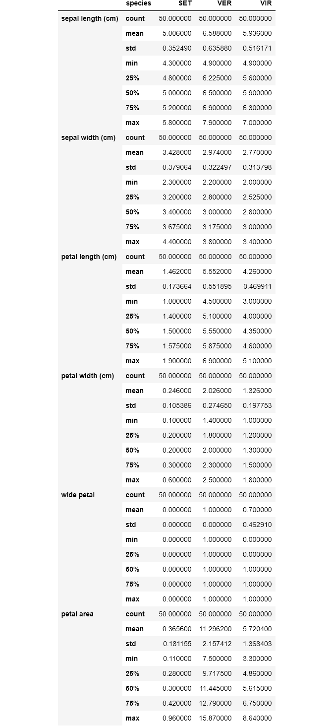

Now we have the total statistics breakdown. When visualizing, we noticed that there are some boundaries setting petal width and petal length of each species apart. So let's explore how we may use groupby to see that;

现在我们有了统计总数。 可视化时，我们注意到有一些边界将每种物种的petal width和petal length分开。 因此，让我们探究如何使用groupby来看到这一点。

# Group the classes by the petal width they are associated withdf.groupby('petal width (cm)')['species'].unique().to_frame()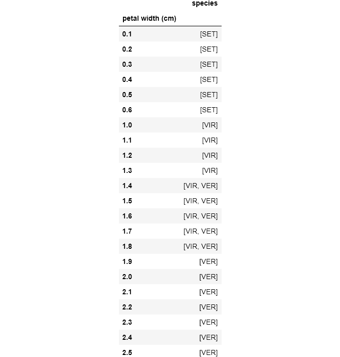

So here, we grouped the species by petal width, another step we could try (as an exercise) is to partition the data into brackets using apply.

因此，在这里，我们根据petal width对species了分组，我们可以尝试的另一步骤(作为练习)是使用apply将数据划分为括号。

Finally, let’s have a look at a custom aggregation function.

最后，让我们看一下自定义聚合函数。

df.groupby('species')['petal width (cm)'].agg(lambda x: x.max() - x.min())# OUTPUT
species
SET    0.5
VER    1.1
VIR    0.8
Name: petal width (cm), dtype: float64

Here, we grouped petal width by species and used a lambda function to get the difference between the maximum petal width and the minimum petal width.

在这里，我们按species petal width进行分组，并使用lambda函数获得最大petal width和最小petal width之间的差。

Note that we’ve scratched at the surfaces of groupby and the other Pandas functions. I greatly encourage you to check out the documentation and learn more about the workings of Pandas.

请注意，我们已经涉及了groupby和其他Pandas函数的表面。 我非常鼓励您查看文档并了解有关Pandas工作原理的更多信息。

建模与评估 (Modeling and Evaluation)

Now that you’ve had a solid understanding of how to manipulate and prepare data, we’ll move on to the next step, which is Modeling.

现在，您已经对如何操作和准备数据有了深刻的了解，我们将继续下一步，即建模。

Here, we’ll discuss the primary Python libraries being used for Machine Learning.

在这里，我们将讨论用于机器学习的主要Python库。

统计模型 (Statsmodels)

Statsmodels is a Python package built for exploring data, estimating models, and running statistical tests. Here, we will use it to build a simple Linear Regression model of the relationship between the sepal length and sepal width of the setosa species.

Statsmodels是一个Python软件包，用于探索数据，估计模型和运行统计测试。 在这里，我们将使用它来建立一个简单的线性回归模型，该模型反映了setosa树的sepal length和sepal width之间的关系。

Let’s create a scatterplot for visual inspection of the relationship;

让我们创建一个散点图以直观检查关系。

plt.figure(figsize=(7,7))
plt.scatter(df['sepal width (cm)'][:50], df['sepal length (cm)'][:50])
plt.xlabel('Sepal Width')
plt.ylabel('Sepal Length')
plt.title('Setosa Sepal Width vs. Length', fontsize=14, y=1.02)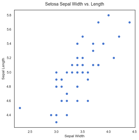

We can see that there’s a positive linear relationship between the two features. The sepal width increases as the sepal length increases. The next step is to run a linear regression on the data using statsmodels to estimate the strength of the relationship.

我们可以看到两个特征之间存在正线性关系。 萼片宽度随着萼片长度的增加而增加。 下一步是使用statsmodels对数据进行线性回归以估计关系的强度。

import statsmodels.api as smy = df['sepal length (cm)'][:50]
x = df['sepal width (cm)'][:50]
X = sm.add_constant(x)results = sm.OLS(y, X).fit()
results.summary()

OLS Regression Results Dep. Variable: sepal length (cm) R-squared: 0.551 Model: OLS Adj. R-squared: 0.542 Method: Least Squares F-statistic: 58.99 Date: Tue, 18 Aug 2020 Prob (F-statistic): 6.71e-10 Time: 18:57:12 Log-Likelihood: 1.7341 No. Observations: 50 AIC: 0.5319 Df Residuals: 48 BIC: 4.356 Df Model: 1 Covariance Type: nonrobust coef std err t P>|t| [0.025 0.975] const 2.6390 0.310 8.513 0.000 2.016 3.262 sepal width (cm) 0.6905 0.090 7.681 0.000 0.510 0.871 Omnibus: 0.274 Durbin-Watson: 2.542 Prob(Omnibus): 0.872 Jarque-Bera (JB): 0.464 Skew: -0.041 Prob(JB): 0.793 Kurtosis: 2.535 Cond. №34.3

OLS回归结果部。 变量：萼片长度(cm)R平方：0.551型号：OLS调整 R平方：0.542方法：最小二乘F统计量：58.99日期：星期二，2020年8月18日Prob(F统计量)：6.71e-10时间：18:57:12对数似然：1.7341观测值：50 AIC ：0.5319 Df残差：48 BIC：4.356 Df模型：1协方差类型：nonrobust coef std err t P> | t | [0.025 0.975] const 2.6390 0.310 8.513 0.000 2.016 3.262萼片宽度(cm)0.6905 0.090 7.681 0.000 0.510 0.871总体：0.274 Durbin-Watson：2.542 Prob(总括)：0.872 Jarque-Bera(JB)：0.464偏斜：-0.041 Prob( JB)：0.793峰度：2.535 Cond。 №34.3

Warnings:[1] Standard Errors assume that the covariance matrix of the errors is correctly specified.

警告：[1]标准错误假设正确指定了错误的协方差矩阵。

Now, here’s the results of our simple regression model. Since this is a linear regression, the model takes the format of Y = B0+ B1X, where B0 is constant (or intercept), and B1 is the regression coefficient. Here, the formula would be Sepal Length = 2.6447 + 0.6909 * Sepal Width. We can also see that the R2 for the model is a respectable 0.558, and the p-value, (Prob), is quite significant.

现在，这是我们简单的回归模型的结果。 由于这是线性回归，因此模型采用Y = B0+ B1X的格式，其中B0是常数(或截距)，而B1是回归系数。 在这里，公式为Sepal Length = 2.6447 + 0.6909 * Sepal Width 。 我们还可以看到，该模型的R2是可观的0.558，并且p-value (Prob)非常重要。

plt.figure(figsize=(7,7))
plt.plot(x, results.fittedvalues, label='regression line', color='r')
plt.scatter(x, y, label='data point')
plt.ylabel('Sepal Length (cm)')
plt.xlabel('Sepal Width (cm)')
plt.title('Setosa Sepal Width vs. Sepal Length', fontsize=14,)
plt.legend(loc=0)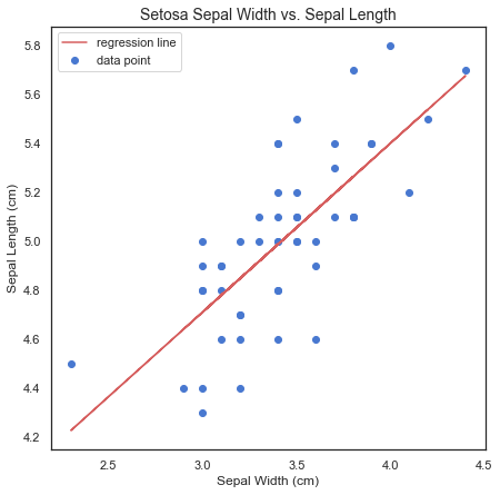

Plotting results.fittedvalues gets us the resulting regression line from our regression.

绘制result.fittedvalues可以从回归中获得回归线。

There are a number of other statistical functions and tests in the statsmodels package, but this by far, the most commonly-used test.

statsmodels软件包中还有许多其他统计功能和测试，但这是迄今为止最常用的测试。

Let’s now move on to the kingpin of Python machine learning packages; All Hail Scikit-learn!

现在让我们继续学习Python机器学习包的主力。 冰雹Scikit的所有学习！

Scikit学习 (Scikit-Learn)

Scikit-learn is an amazing Python library with outstanding documentation, designed to provide a consistent API to dozens of algorithms. It is built upon and is itself, a core component of the Python scientific stack, which includes NumPy, SciPy, Pandas, and Matplotlib. Here are some of the areas scikit-learn covers: classification, regression, clustering, dimensionality reduction, model selection, and preprocessing.

Scikit-learn是一个了不起的Python库，具有出色的文档，旨在为许多算法提供一致的API。 它建立在Python科学堆栈的核心组件之上，并且本身就是它的核心组件，其中包括NumPy，SciPy，Pandas和Matplotlib。 scikit学习的领域包括：分类，回归，聚类，降维，模型选择和预处理。

Now, let’s build a classifier with our iris data, and then we’ll look at how we can evaluate our model using the tools of scikit-learn:

现在，让我们用虹膜数据构建一个分类器，然后看一下如何使用scikit-learn工具评估模型：

1. The data should be split into the predictors and the target; The predictors (independent variables) should be a numeric n * m matrix, X, and the target (dependent variable), y, an n * 1 vector.

   数据应分为预测变量和目标变量； 预测变量(独立变量)应为数字n * m矩阵X，目标变量应为y n * 1向量。

2. These are then passed into the .fit() method on the chosen classifier.

   然后将它们传递到所选分类器的.fit()方法中。

3. And then we can use .predict() method to make predictions on new data.

   然后，我们可以使用.predict()方法对新数据进行预测。

This is the greatest benefit of using scikit-learn: each classifier utilizes the same methods to the extent possible. This makes swapping them in and out a breeze. We’ll see this in action soon.

这是使用scikit-learn的最大好处：每个分类器都尽可能利用相同的方法。 这使得轻松地将它们交换进出。 我们很快就会看到这个动作。

from sklearn.model_selection import train_test_split as ttsy = df.pop('species')
X_train, X_test, y_train, y_test = tts(df, y, test_size=.3)from sklearn.ensemble import RandomForestClassifierclf = RandomForestClassifier(max_depth=5, n_estimators=10)clf.fit(X_train, y_train)
y_pred = clf.predict(X_test)rf = pd.DataFrame(list(zip(y_pred, y_test)), columns=['predicted', 'actual'])
rf['correct'] = rf.apply(lambda x: 1 if x.predicted == x.actual else 0, axis=1)
rf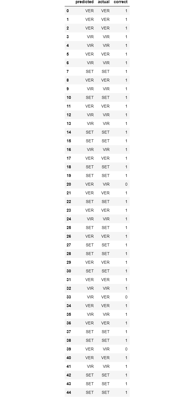

Now let’s run this line of code;

现在让我们运行这一行代码；

# accuracy percentagerf['correct'].sum() / rf['correct'].count()# OUTPUT
0.9333333333333333

In the preceding lines of code, we’ve built, trained, and tested a classifier with a 93% accuracy level on our iris dataset. Now let’s go through each step one by one;

在前面的代码行中，我们在虹膜数据集上构建，训练和测试了分类器，分类器的准确度为93％。 现在，让我们一步一步地完成每个步骤；

• We imported train_test_split from scikit-learn, which is shortened to sklearn the import statement. train_test_split is a module for splitting data into training and testing sets. This is a very important practice in building models. We'd train our model with the training set and validate our model's performance with the testing set.

  我们从scikit-learn导入train_test_split ，将其缩短为sklearn import语句。 train_test_split是用于将数据分为训练和测试集的模块。 这是建立模型中非常重要的做法。 我们将使用训练集来训练模型，并使用测试集来验证模型的性能。

• In the 2nd line, we separated the target variable, which is species, from the predictors. (In mathematical lingua, we created our X matrix and our y vector)

  在第二行中，我们将目标变量( species )与预测变量分开。 (在数学语言中，我们创建了X矩阵和y向量)

• Then we used train_test_split to split the data. As you'd notice, we set test_size to 0.3, which means that the testing set should be 30% of the whole data. The train_test_split module also shuffles our data, as the order may contain bias which we won't want the model to learn.

  然后，我们使用train_test_split拆分数据。 您会注意到，我们将test_size设置为0.3，这意味着测试集应为整个数据的30％。 train_test_split模块还对我们的数据进行train_test_split ，因为该顺序可能包含我们不希望模型学习的偏差。

• Moving to the next cell, we imported a Random Forest Classifier from the sklearn module. we instantiated our forest classifier in the next line using 10 Decision Trees, and each tree has a maximum split depth of five, in a bid to avoid overfitting.

  移至下一个单元格，我们从sklearn模块导入了一个随机森林分类器。 为了避免过度拟合，我们在下一行使用10个决策树实例化了森林分类器，每棵树的最大拆分深度为5。

• Next, our model is fitted using the training data. Having trained our classifier, we called the predict method on our classifier passing in our test data. Remember that the test data is the data that the classifier has not seen yet.
  接下来，使用训练数据拟合我们的模型。 训练完分类器后，我们在传递测试数据的分类器上调用了预报方法。 请记住，测试数据是分类器尚未看到的数据。
• We then created a DataFrame of the actual labels vs the predicted labels. Afterward, we totaled the correct predictions and divide them by the total number of instances, which then gave us a very high accuracy.
  然后，我们创建了实际标签与预测标签的DataFrame。 之后，我们对正确的预测进行总计，然后将其除以实例总数，从而获得了非常高的准确性。

Let’s now see the features that gave us the highest predictive power;

现在让我们看看赋予我们最高预测能力的功能；

# Feature Selectionf_names = df.columns
f_importances = clf.feature_importances_
f_std = np.std([tree.feature_importances_ for tree in clf.estimators_], axis=0)zz = zip(f_names, f_importances, f_std)
zzs = sorted(zz, key=lambda x: x[1], reverse=True)labels = [x[0] for x in zzs]
imps = [x[1] for x in zzs]
errs = [x[2] for x in zzs]plt.figure(figsize=(10,4))
plt.bar(range(df.shape[1]), imps, color='r', yerr=errs, align='center')
plt.xticks(range(len(f_importances)), labels)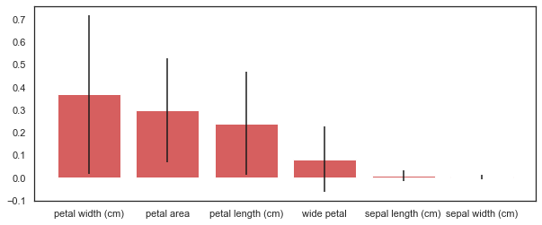

As we expected, based upon our earlier visual analysis, the petal length and width have more discriminative power when differentiating between the iris classes.

正如我们所期望的，基于我们较早的视觉分析，在区分虹膜类别时，花瓣的长度和宽度具有更大的判别力。

And as I mentioned when we checked the correlation between our features, sepal length and sepal width seem to contribute very little to our model’s accuracy.

正如我提到的，当我们检查特征之间的相关性时，萼片长度和萼片宽度似乎对模型精度的影响很小。

How did we get this? The random forest has a method called .feature_importances_ that returns the relative performance of the feature for splitting at the leaves. If a feature is able to consistently and cleanly split a group into distinct classes, it will have high feature importance.

我们是怎么得到的？ 随机森林具有一种称为.feature_importances_的方法，该方法返回用于在叶子处进行分割的要素的相对性能。 如果某个功能能够始终如一地将一个组清晰地划分为不同的类，那么它将具有很高的功能重要性。

You’d notice that we included the standard deviation, which helps to illustrate how consistent each feature is. This is generated by taking the feature importance, for each of the features, for each of the ten trees, and calculating the standard deviation.

您会注意到我们包含了标准偏差，这有助于说明每个功能的一致性。 这是通过针对十个树中的每个特征，针对每个特征并选择标准偏差来得出特征重要性的。

Let’s now take a look at one more example using Scikit-learn. We will now switch out our classifier and use a support vector machine (SVM):

现在让我们看一下使用Scikit-learn的另一个示例。 现在，我们将切换分类器，并使用支持向量机(SVM) ：

from sklearn.multiclass import OneVsRestClassifier
from sklearn.svm import SVCclf = OneVsRestClassifier(SVC(kernel='linear'))clf.fit(X_train, y_train)
y_pred = clf.predict(X_test)svc = pd.DataFrame(list(zip(y_pred, y_test)), columns=['predicted', 'actual'])
svc['correct'] = svc.apply(lambda x: 1 if x.predicted == x.actual else 0, axis=1)
svc

Now let’s execute the following line of code;

现在，让我们执行以下代码行；

svc['correct'].sum() / svc['correct'].count()# OUTPUT
0.9333333333333333

Here we used SVM instead of Random Forest Classifier without changing any of our code, except for the part where we imported in Support Vector Classifier and instantiated the model. This is just a taste of the unparalleled power that Scikit-learn offers.

在这里，我们使用SVM而不是随机森林分类器，而无需更改任何代码，除了在支持向量分类器中导入并实例化模型的部分。 这只是对Scikit-learn提供的无与伦比的力量的一种体验。

I’d strongly suggest that you’d go to the Scikit-learn docs and check out some of the other ML algorithms that Scikit-learn has to offer.

我强烈建议您去Scikit-learn文档，并查看Scikit-learn必须提供的其他ML算法。

最后说明 (Final Notes)

With this, we’re done with this introductory guide to Data Analysis and Machine Learning.

这样，我们就完成了本数据分析和机器学习入门指南。

In this article, we learned how to take our data, step by step, through each stage of Data Analysis and Machine Learning. We also learned the key features of each of the primary libraries in the Python scientific stack.

在本文中，我们学习了如何通过数据分析和机器学习的每个阶段逐步获取数据。 我们还学习了Python科学堆栈中每个主要库的关键功能。

Here is the link to the code and explanations on GitHub.

这是GitHub上的代码和说明的链接 。

In subsequent articles, we will take this knowledge and begin to apply them to create unique and useful machine learning applications. Stay tuned!

在随后的文章中，我们将掌握这些知识并开始将其应用到创建独特且有用的机器学习应用程序中。 敬请关注！

Meanwhile, like and share this article if you find it insightful. You may also say hi to me on Twitter and LinkedIn. Have fun!

同时，如果您发现本文很有见地，请喜欢并分享本文。 您也可以在Twitter和LinkedIn上对我问好 。 玩得开心！

Note: This article was heavily inspired by Python Machine Learning Blueprints by Alexander T. Combs.

注意：本文的主要灵感来自Alexander T. Combs的Python机器学习蓝图 。

翻译自: https://levelup.gitconnected.com/practical-guide-into-data-analysis-and-machine-learning-using-python-7e8ce4081dfc