lstm 利率预测_用武器预测利率

lstm 利率预测

Wall Street indices predicted nine out of the last five recessions ~ Paul A. Samuelson

华尔街指数预测最近五次衰退中有九次〜Paul A. Samuelson

The quote above explains why correctly forecasting something is just another word for getting lucky but forecasting interest rates in particular has been the point of interest for many researchers and mathematicians for some time now. While many contributors have extended the ARMA model to better forecast interest rates, this post aims to provide an introduction to the sea of research with a very basic but a very strong model.

上面的引言解释了为什么正确地预测事物只是获得幸运的另一种说法，但是在一段时间以来，尤其是预测利率一直是许多研究人员和数学家的关注点。 尽管许多贡献者已将ARMA模型扩展到更好地预测利率，但本文旨在通过一个非常基本但非常强大的模型向研究海洋介绍。

The Auto-Regressive (AR) Moving-Average (MA) model has two things going on simultaneously. The ‘AR’ part of the model regresses the data on its own past values, using the history of the variable to predict its future movements. The ‘MA’ part of the model learns from lagged error terms, or the white-noise in the past values of the variable.

自回归(AR)移动平均(MA)模型同时进行了两件事。 该模型的“ AR”部分使用变量的历史记录来预测其未来的移动，从而根据自己的过去值对数据进行回归。 该模型的“ MA”部分从滞后误差项或变量的过去值中的白噪声中学习。

The first summation takes into account the AR part of the model for ‘p’ values of lag whereas the second summation accounts for the MA part with ‘q’ values of lag. ε is the error term for ‘q’ lagged values. φ is the AR coefficient and θ is the MA coefficient. The AR and MA coefficients take values upon training on the data provided to the model.

第一个求和考虑了模型的AR部分的“ p”个滞后值，而第二个求和考虑了具有“ q”个值的滞后的MA部分。 ε是“ q”滞后值的误差项。 φ是AR系数，θ是MA系数。 在对提供给模型的数据进行训练时，AR和MA系数取值。

使用正确的数据 (Using the Right Data)

As a first step, I’ll be importing my data.

第一步，我将导入数据。

#Importing Library
import pandas as pdfrom pandas.plotting import register_matplotlib_converters
register_matplotlib_converters() #allows using dates for indexing#Importing Datadf = pd.read_csv (r'path of file', parse_dates=['DATE'],   index_col=['DATE'])FFR = df['FFR'].dropna()

You can download this .csv file from here. With the data loaded, we’ll have to check for its stationarity before plugging it into an ARMA model.

您可以从此处下载此.csv文件。 加载数据后，我们必须在将其插入ARMA模型之前检查其平稳性。

What differentiates ARMA from ARIMA is that an ARIMA model is able to handle non-stationary data. In this post, however, we’ll be using an ARMA model and I will therefore leave the debate of handling non-stationary data for another post.

ARMA与ARIMA的区别在于ARIMA模型能够处理非平稳数据。 但是，在这篇文章中，我们将使用ARMA模型，因此我将在另一篇文章中讨论处理非平稳数据的争论。

But this doesn’t mean we can feed non-stationary data into an ARMA model and hope for great results, and interest rates data is almost never stationary. For this reason, I will be using the monthly Federal Funds interest rate data from 2009 to 2020, which happens to exhibit a good degree of stationarity.

但这并不意味着我们可以将非平稳数据输入到ARMA模型中并希望取得良好结果，而利率数据几乎永远不会停止。 因此，我将使用2009年至2020年的每月联邦基金利率数据，该数据显示出良好的平稳性。

import matplotlib.pyplot as pltplt.plot(FFR)
plt.title ('Feds Funds Rate')
plt.xlabel ('Year')
plt.show()

How do I know it’s stationary? I don’t! Until you use a statistical method to estimate stationarity, you cannot establish that you can move forward with your data. A common method to use is the ADF test. The ADF test gives you two kinds of results:

我怎么知道它是静止的？ 我不！ 在使用统计方法估计平稳性之前，您无法确定可以继续使用数据。 常用的方法是ADF测试。 ADF测试为您提供两种结果：

1. The p-value:

   p值：

   p-value ≤ 0.05 means that data is stationary

   p值≤0.05表示数据是固定的

   p-value > 0.05 means it’s not stationary

   p值> 0.05表示它不是固定的

2. The ADF Statistic

   ADF统计

   If the ADF Statistic < 1% critical value it means you can reject the hypothesis (that your data is non-stationary) with a significance level of 1%.

   如果ADF统计量<1％临界值，则意味着您可以以1％的显着性水平拒绝该假设(您的数据是非平稳的)。

   Similarly, ADF statistic can be compared against a variety of significance levels.

   同样，可以将ADF统计与各种显着性水平进行比较。

In Python, StatsModels allows for a quick and easy way to estimate stationarity of data using the ADF test.

在Python中，StatsModels允许使用ADF测试快速简便地估算数据的平稳性。

from statsmodels.tsa.stattools import adfullerresult = adfuller(FFR)
print('ADF Statistic: %f' % result[0])
print('p-value: %f' % result[1])
print('Critical Values:')
for key, value in result[4].items():
    print('\t%s: %.3f' % (key, value))

Given that the p-value is less than 0.05 and that the ADF Statistic is less than the 1% critical value, we can establish with some certainty that our data is stationary.

假设p值小于0.05，并且ADF统计量小于1％临界值，则可以确定我们的数据是固定的。

训练ARMA模型 (Training the ARMA Model)

Now that our data is ready to use, let’s see how the ARMA model works.

现在我们的数据已经可以使用了，让我们看看ARMA模型是如何工作的。

Here I’ll be using an ARMA (1,0) model. A model which regresses 1 lagged value of the Fed’s Funds Rate and 0 lagged terms for the moving average.

在这里，我将使用ARMA(1,0)模型。 该模型将美联储基金利率的1个滞后值与移动平均值的0个滞后项进行回归。

# Importing the ARMA Library
from statsmodels.tsa.arima_model import ARMA# Training Forecast Model with FFR Data using ARMA(1,0)
model_1 = ARMA(FFR, order=(1,0))
ffr_pred = model_1.fit()
print(ffr_pred.summary())

The summary of the model can give some important numbers that help you understand how well your model performed. The summary of this model looks like this

模型的摘要可以提供一些重要的数字，以帮助您了解模型的性能。 该模型的摘要如下所示

Lower AIC, BIC and HQIC values tell you that your model predicted values closer to the truth. Log Likelihood is an estimate of the fitness of the model, higher log likelihood values are desirable. ‘const’ is the constant ‘c’ added to every observation predicted by the model, in simpler words, it works like a lower bound if all other values in the model are non-negative. ‘ar.L1.FFR’ is the AR coefficient φ. We don’t see the MA coefficient θ because we used 0 MA terms to predict values in the model. From the summary we can infer that:

较低的AIC，BIC和HQIC值表明，您的模型预测值更接近真实情况。 对数似然度是模型适用性的估计，需要较高的对数似然值。 'const'是在模型预测的每个观察值中添加的常数'c'，用简单的话来说，如果模型中的所有其他值均为非负数，则它像下限一样工作。 “ ar.L1.FFR”是AR系数φ。 我们看不到MA系数θ，因为我们使用0个MA项来预测模型中的值。 从总结中我们可以推断出：

c = 0.3657φ = 0.9846

c =0.3657φ= 0.9846

Now, let’s test the model by forecasting some values.

现在，让我们通过预测一些值来测试模型。

# Plot the original series and the forecasted series
ffr_pred_endog.plot_predict(start=90, end=134)
plt.legend(fontsize=8)
plt.title('Forecasted FFR vs Actual FFR ')
plt.savefig('ffr forecast')
plt.show()

Sklearn in Python gives us a convenient function to calculate the accuracy of our model.

Python中的Sklearn为我们提供了一个方便的函数来计算模型的准确性。

#Calculating Accuracy 
from sklearn import metricsacc_1_pred = ffr_pred.predict(start=90, end=134)
acc_1_true = FFR[-len(acc_1_pred):]print('Mean Squared Error = ' , metrics.mean_squared_error(acc_1_true , acc_1_pred))
print('Mean Absolute Error = ' , metrics.mean_absolute_error(acc_1_true , acc_1_pred))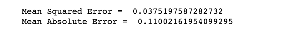

MSE of 0.037 is a fairly low error value to move forward with.

MSE为0.037，这是一个相当低的误差值，可以继续前进。

We could also use this model to forecast future FFR values.

我们还可以使用此模型来预测未来的FFR值。

#Forecasting Future Values for 24 Months ffr_pred.plot_predict(start=135 , end=159, dynamic= True)ffr_forecast = np.array(ffr_pred.predict(start=135, end=159))

Appending the results with the actual past values looks like this.

将结果与实际过去的值相加看起来像这样。

The best we can do to test the accuracy of future forecasted values is by comparing them with the results of other people. The US Federal Reserve gives an FOMC projection for a number of economic variables in an annual report which should make it a reliable source to test the results of our model with. You can find the report here. We can see constantly near-zero values of the Fed’s Funds Rate here as our model predicted.

我们最好的测试未来预测值准确性的方法是将它们与其他人的结果进行比较。 美联储在年度报告中提供了FOMC对许多经济变量的预测，这将使其成为检验我们模型结果的可靠来源。 您可以在这里找到报告。 正如我们的模型所预测的，我们可以在这里看到美联储基金利率一直接近零的值。

Source: federalreserve.gov

资料来源：Federalreserve.gov

The purpose of this post and methodology is to give you a glance on how Python can be used for forecasting variables, any consequential decisions should be followed by proper research and understanding.

这篇文章和方法的目的是让您了解如何使用Python预测变量，任何后续决定都应经过适当的研究和理解。

翻译自: https://medium.com/@syedhadi816/forecasting-interest-rates-with-arma-649cbcd2d388

lstm 利率预测