预测性维护_工厂数据的预测性维护

最新推荐文章于 2024-04-13 11:59:08 发布

weixin_26750511

最新推荐文章于 2024-04-13 11:59:08 发布

阅读量1.6k

点赞数 3

文章标签： java python

原文链接：https://medium.com/@andrey.i.karpov/predictive-maintenance-on-factory-data-4f8cc17696e4

版权

预测性维护

In the era of digitization the concept of Smart Factory attracts a lot of attention. Modern industry becomes connected and highly automated. Such factories need their machines to run smoothly and with minimal down times. Predictive maintenance helps to deal with breakages. It aims to identify possible failures and helps to schedule the maintenance of detected devices.

在数字化时代，智能工厂的概念吸引了很多关注。现代工业变得互联且高度自动化。这样的工厂需要他们的机器运行平稳，停机时间最少。预测性维护有助于处理破损。它旨在识别可能的故障并帮助安排检测到的设备的维护。

In current blog post I illustrate the process of building a model that detects failures of factory machines. I use an open dataset from one of the Schwan’s factories. It contains time series values that include telemetry, device errors and failures. The aim is to predict device failure 12 hours before it happens. An assumption is that half of a day is enough for a technician to react and to handle a possible issue.

在当前的博客文章中，我说明了构建检测工厂机器故障的模型的过程。我使用Schwan一家工厂的开放数据集。它包含时间序列值，包括遥测，设备错误和故障。目的是在发生故障前12小时预测设备故障。假设半天时间足以使技术人员做出React并解决可能的问题。

探索数据集 (Exploring dataset)

The first thing to do is reading the dataset and loading data into pandas data frames. This logic is quite trivial, so I do not post it here. Instead you can access the original Jupyter Notebook at this link.

首先要做的是读取数据集并将数据加载到熊猫数据框中。这种逻辑非常琐碎，因此我不在此发布。相反，您可以通过此链接访问原始的Jupyter Notebook。

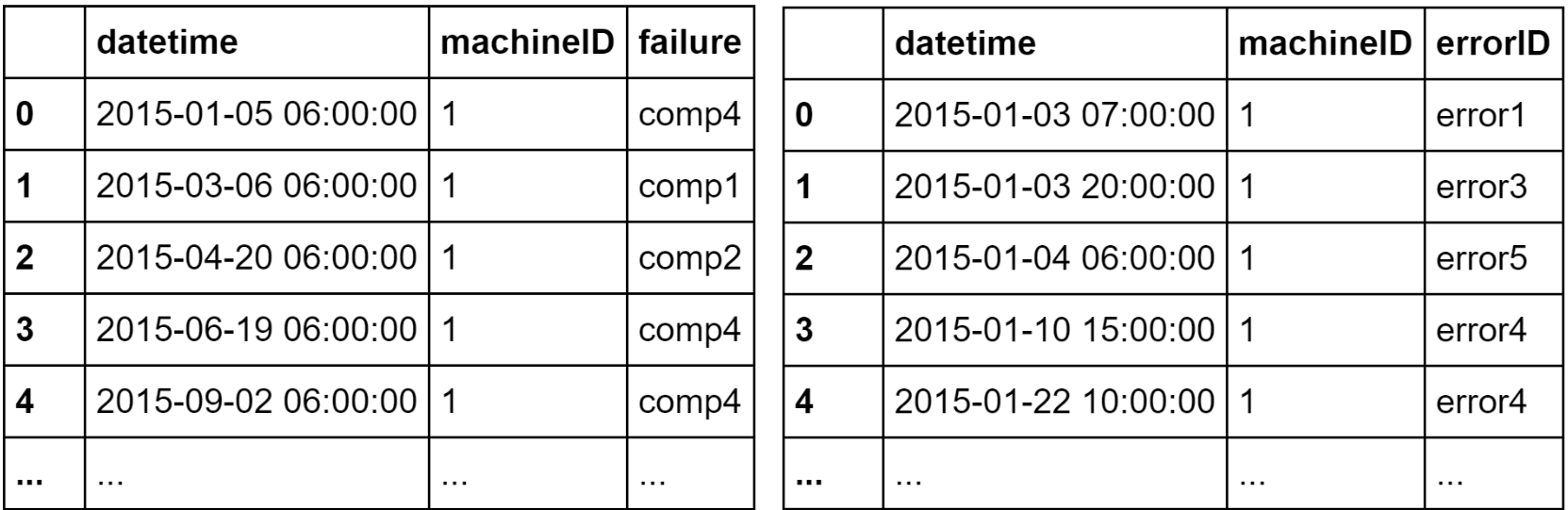
In general there are 3 files to read: telemetry.csv, failures.csv and errors.csv. At the end we get 3 pandas data frames: telemetry_df, failures_df and errors_df.

通常，有3个文件需要读取：telemetry.csv，failures.csv和errors.csv。最后，我们得到3个熊猫数据帧：telemetry_df，failures_df和errors_df。

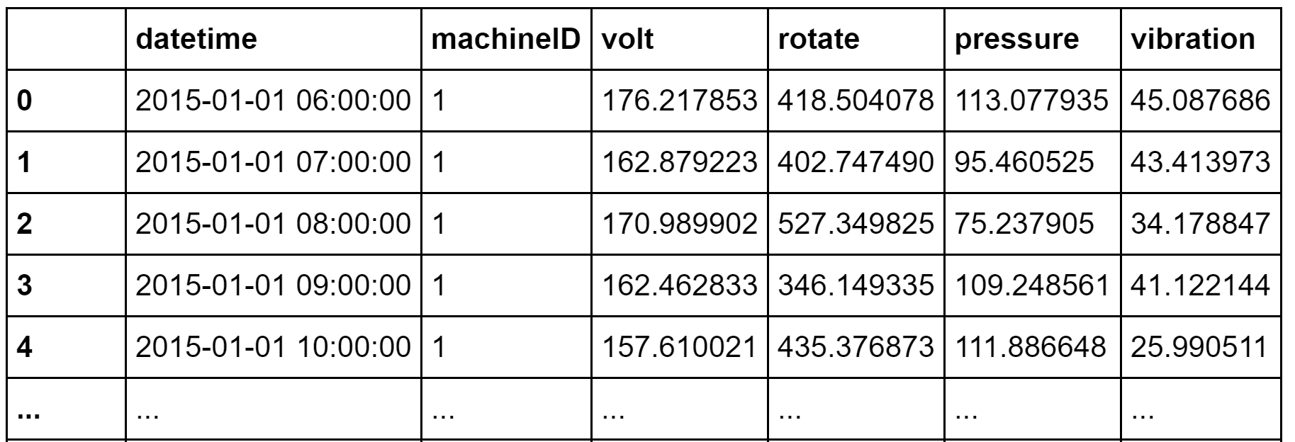
In total there are 876100 rows of telemetry values for 100 machines during 1 year on an hour basis. This is a lot, but most of the time devices work well. All in all the data set contains only 3919 errors and 761 failures. The latest are the values we try to predict.

在1年中，以小时为单位，总共有100台机器的876100行遥测值。这很多，但是大多数时候设备运行良好。所有数据集总共仅包含3919个错误和761个失败。最新是我们尝试预测的值。

We have data for 100 machines. In real predictive maintenance cases it often makes sense to create a separate model for each machine for having best predictions. In this example we assume that one model might work for all the devices. To check it, let’s build box plots for telemetry values of all machines and compare their distributions.

我们有100台机器的数据。在实际的预测性维护案例中，通常有必要为每台机器创建一个单独的模型以实现最佳预测。在此示例中，我们假设一个模型可能适用于所有设备。要检查它，让我们为所有机器的遥测值构建箱形图并比较它们的分布。

import matplotlib.pyplot as plt
import numpy as np


volt_values = []
rotate_values = []
pressure_values = []
vibration_values = []

for i in range(1,101):
    volt_values.append(telemetry_df[telemetry_df['machineID'] == i]["volt"])
    rotate_values.append(telemetry_df[telemetry_df['machineID'] == i]["rotate"])
    pressure_values.append(telemetry_df[telemetry_df['machineID'] == i]["pressure"])
    vibration_values.append(telemetry_df[telemetry_df['machineID'] == i]["vibration"])

    
fig, axs = plt.subplots(4, 1, constrained_layout=True, figsize=(18, 16))
fig.suptitle('Telemetry values per machine', fontsize=16)


def build_box_plot(plot_index, plot_values, title):
    axs[plot_index].boxplot(plot_values)
    axs[plot_index].set_title(title)
    axs[plot_index].set_xticks([1, 26, 51, 76, 101])
    axs[plot_index].set_xticklabels([1, 25, 50, 75, 100])

    
build_box_plot(0, volt_values, "Volt")
build_box_plot(1, rotate_values, "Rotate")
build_box_plot(2, pressure_values, "Pressure")
build_box_plot(3, vibration_values, "Vibration")
plt.show()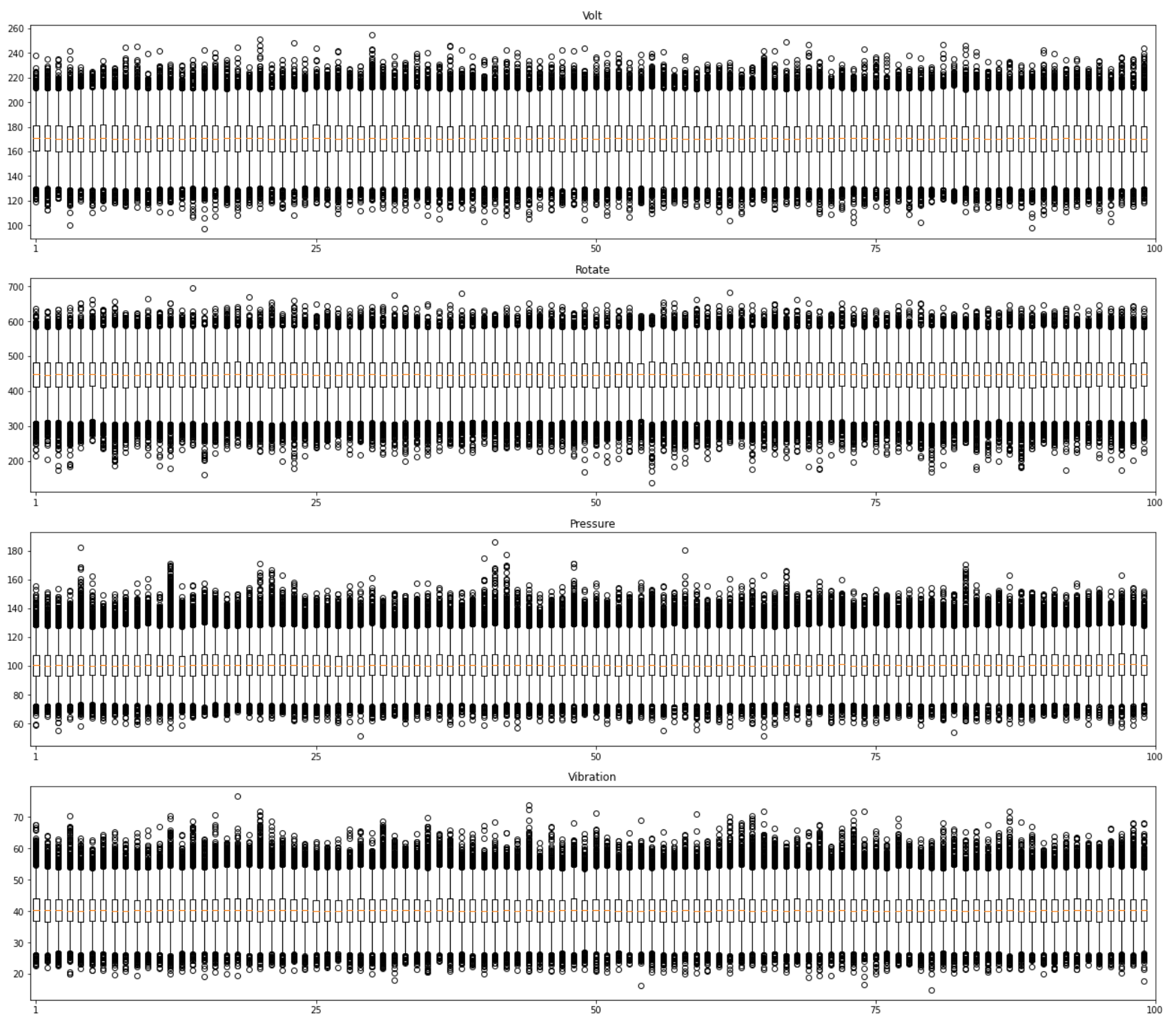

The picture above show us that all machines have approximately same distributions of their telemetry values. So, we might assume that they are similar from the technical point of view and hence we can train one model for all of them.

上图显示了所有机器的遥测值分布大致相同。因此，我们可以假设从技术角度来看它们是相似的，因此我们可以为所有模型训练一个模型。

Of course it’s still hard to decide if our data is sufficient for predicting failures. So, we need to explore it further. Now we combine all 3 data frames into one (see the original notebook) and build scatter plots for pairs “Rotate-Volt” and “Vibration-Pressure”. We also mark the failure cases in red. By doing this we want to check if failures are grouped together or occur for extreme values known as outliers.

当然，仍然很难确定我们的数据是否足以预测故障。因此，我们需要进一步探索。现在，我们将所有3个数据帧组合为一个(请参阅原始笔记本)，并为“旋转-电压”和“振动-压力”对建立散点图。我们还将失败案例标记为红色。通过执行此操作，我们要检查是否将故障分组在一起或是否发生了称为异常值的极端值。

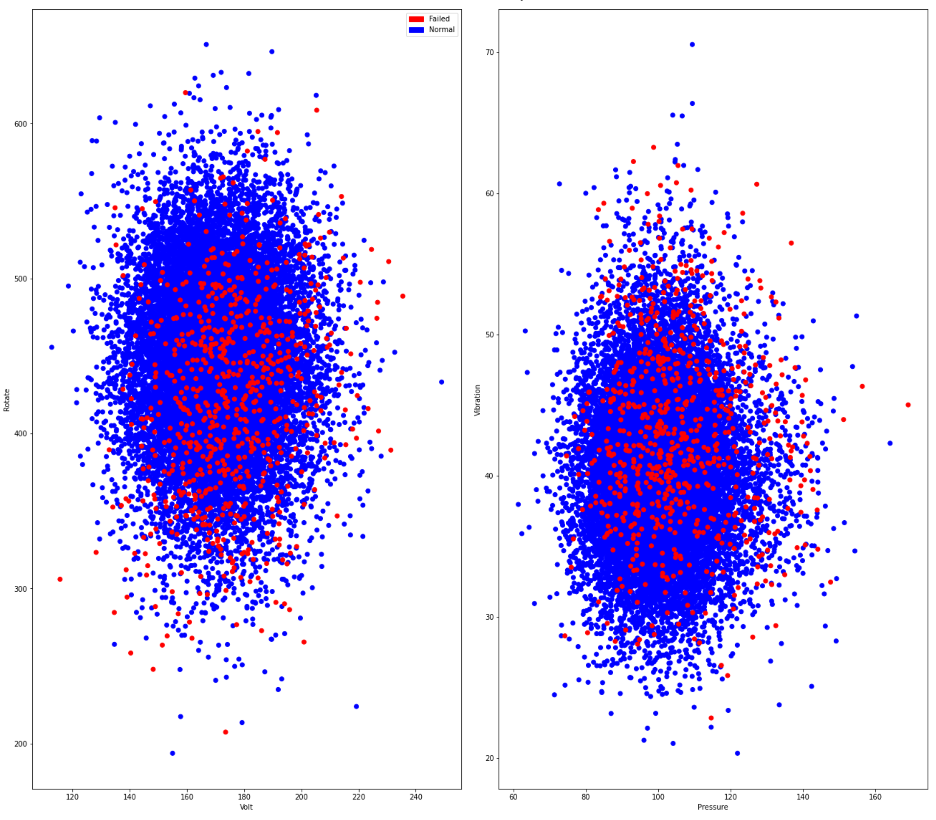
Looking at the plots we might conclude that there are simple patterns. It does not mean that telemetry is useless. But it tells us that it won’t be a straight forward and good predictor as it is. From the other side there still can be complex patterns especially in the way how values behave over time. These patterns cannot be seen on simple plots but still can be detected by non-linear models.

查看这些图，我们可能会得出结论：存在简单的模式。这并不意味着遥测是无用的。但是它告诉我们，它不会是一个简单明了的预测者。另一方面，仍然存在复杂的模式，尤其是在值随时间变化的方式上。这些模式无法在简单的图上看到，但仍可以通过非线性模型检测到。

Now let’s explore errors. They might happen some time before the failures and be a good indicator. To check them we first randomly sample 6 failure cases. Then we pick a time frame of 48 hours before the failure. Plots below show both telemetry values and errors that are marked by red lines.

现在让我们探索错误。它们可能在故障发生前的某个时间发生，并且是一个很好的指示。为了检查它们，我们首先随机抽样6个失败案例。然后我们选择故障发生前48小时的时间范围。下面的图显示了遥测值和用红线标记的错误。

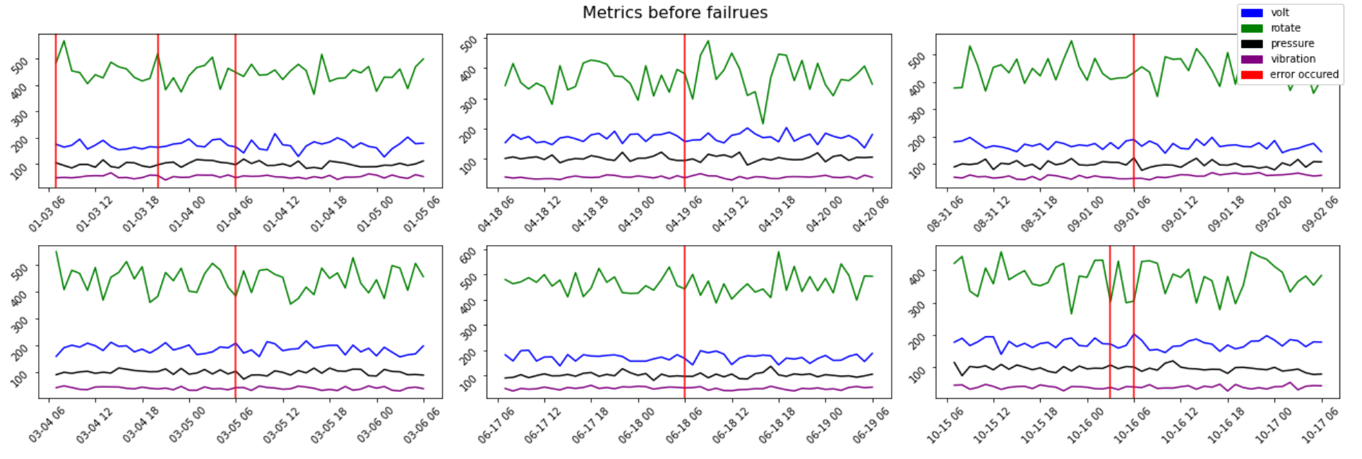
In all 6 examples there are errors that happen several hours before the actual failure. So, they might be a good predictor.

在所有6个示例中，都存在在实际故障发生前几个小时发生的错误。因此，它们可能是一个很好的预测指标。

准备数据集 (Prepare dataset)

After exploring dataset we have several assumptions:

探索数据集后，我们有几个假设：

We can combine data for all machines and train one model.
我们可以合并所有机器的数据并训练一个模型。
Telemetry is not a good predictor alone, but still might improve the model in some cases. So, we calculate the rolling values and use them during the model training.
遥测本身并不是一个好的预测指标，但在某些情况下仍可以改善模型。因此，我们计算滚动值并在模型训练期间使用它们。
Errors seem to be a good predictor.
错误似乎是一个很好的预测指标。
The number of failures is low comparing to the number of normal functioning samples.
与正常运行的样本数量相比，失败的数量很少。

First of all we need to prepare a dataset for training. Preparation includes:

首先，我们需要准备训练数据集。准备工作包括：

Pick all failure cases
选择所有失败案例
Randomly sample 30000 normal cases
随机抽样30000例正常病例
Subtract 12 hours (predict failure 12 hours before) and pick a time window of 36 hours back.
减去12个小时(预测12个小时之前会发生故障)，然后选择36个小时的时间范围。
Calculate the number of errors of each type during the defined time frame
计算在定义的时间范围内每种类型的错误数
Calculate telemetry statistics (min, max, std, mean) during the defined time frame
在定义的时间范围内计算遥测统计信息(最小，最大，标准，均值)
Split the dataset into train, test and validation
将数据集分为训练，测试和验证

Let’s prepare the column names and a method for calculating statistics.

让我们准备列名和一种计算统计量的方法。

hours_ahead = 12
hours_lag = 36
tel_columns = ["volt", "rotate", "pressure", "vibration"]
error_columns = ["error1", "error2", "error3", "error4", "error5"]

col_names = []
for tel_c in tel_columns:
    col_names.extend([tel_c + "_min", tel_c + "_max", tel_c + "_std", tel_c + "_mean"])

for err_c in error_columns:
    col_names.append(err_c + "_sum")


def get_time_span_statistics(source_df, lag_start, lag_end):
    lag_values_df = source_df.iloc[lag_start:lag_end]
    failure_record = []

    for col_name in tel_columns:
        failure_record.extend([lag_values_df[col_name].min(), 
                               lag_values_df[col_name].max(), 
                               lag_values_df[col_name].std(), 
                               lag_values_df[col_name].mean()])

    for col_name in error_columns:
        failure_record.append(lag_values_df[col_name].sum())
    
    return failure_record

Next step is to calculate values for all failure cases.

下一步是计算所有失败案例的值。

failure_records = []
failure_ranges = []

for f_index in failure_indexes:
    start_i = f_index - hours_ahead - hours_lag
    end_i = f_index - hours_ahead
    
    failure_ranges.extend(np.arange(f_index - hours_ahead - hours_lag, f_index + hours_ahead + hours_lag))
    failure_records.append(get_time_span_statistics(telemetry_df, start_i, end_i))

failure_records_df = pd.DataFrame(failure_records)
failure_records_df.columns = col_names
failure_records_df['is_error'] = True

Sample normal cases and combine them with failures.

对正常情况进行抽样，并将其与故障结合起来。

normal_functioning_records = []
normal_functioning_indexes = telemetry_df.drop(failure_ranges).sample(30000).index

for n_index in normal_functioning_indexes:        
    start_i = n_index - hours_ahead - hours_lag
    end_i = n_index - hours_ahead
    normal_functioning_records.append(get_time_span_statistics(telemetry_df, start_i, end_i))

normal_functioning_records_df = pd.DataFrame(normal_functioning_records)
normal_functioning_records_df.columns = col_names
normal_functioning_records_df['is_error'] = Falsecombined_df = pd.concat([failure_records_df, 
normal_functioning_records_df], ignore_index=True)# shuffle the data set
combined_df = combined_df.sample(len(combined_df))

Now we need to split the combined dataset into train, test and validation subsets.

现在我们需要将合并的数据集分为训练，测试和验证子集。

split_mask = np.random.rand(len(combined_df)) < 0.7

x_df = combined_df.drop(['is_error'], axis=1)
y_df = combined_df['is_error']

x_train = x_df[split_mask]
y_train = y_df[split_mask]

x_test_validation = x_df[~split_mask]
y_test_validation = y_df[~split_mask]

split_mask = np.random.rand(len(x_test_validation)) < 0.5
x_validation = x_test_validation[split_mask]
y_validation = y_test_validation[split_mask]

x_test = x_test_validation[~split_mask]
y_test = y_test_validation[~split_mask]

As a result we have the following subsets:

结果，我们具有以下子集：

Training set: total items = 21379, failure items = 474
训练集：总项= 21379，失败项= 474
Validation set: total items = 4599, failure items = 120
验证集：总项数= 4599，失败项数= 120
Test set: total items = 4741, failure items = 125
测试集：总项数= 4741，失败项数= 125

The subsets are imbalanced. We need to keep it in mind while picking the validation metrics. For example, accuracy is not sufficient. It’s better to look at precision, recall and F1 score.

子集不平衡。在选择验证指标时，我们需要牢记这一点。例如，准确性不足。最好看一下精度，召回率和F1得分。

培训与评估 (Training and evaluation)

After preparing the dataset we are ready to start training. In current example we are going to train a gradient boosting model. This is a quite powerful ensemble algorithm that provides a non-linear classifier. For evaluation we use AUCPR, which is better for imbalanced datasets.

准备好数据集后，我们就可以开始训练了。在当前示例中，我们将训练梯度提升模型。这是一种功能强大的集成算法，可提供非线性分类器。为了进行评估，我们使用AUCPR，这对于不平衡的数据集更好。

from xgboost import XGBClassifier


model = XGBClassifier(max_depth=10, n_estimators=100, seed=0)
model.fit(
    x_train, 
    y_train, 
    eval_set=[(x_validation, y_validation)], 
    early_stopping_rounds=10, 
    eval_metric="aucpr"
)

The training reaches an AUC value of 0.98345, which is a very high result. To get final metrics we need to evaluate the model on the test set that has not been used during the training.

训练达到的AUC值为0.98345，这是非常高的结果。为了获得最终指标，我们需要在训练过程中未使用的测试集上评估模型。

The script below calculates precision, recall, F-score, builds ROC curve and confusion matrix.

下面的脚本计算精度，召回率，F得分，建立ROC曲线和混淆矩阵。

from sklearn import metrics


test_predictions = model.predict(x_test)
precision, recall, fscore, _ = metrics.precision_recall_fscore_support(y_test, test_predictions, average='weighted')

print("Precision {}, Recall {}, F-Score {}".format(precision, recall, fscore))
metrics.plot_roc_curve(model, x_test, y_test)
metrics.plot_confusion_matrix(model, x_test, y_test)

Final scores:

最终成绩：

Precision = 0.99719
精度= 0.99719
Recall = 0.99722
召回= 0.99722
F-Score = 0.99719
F分数= 0.99719

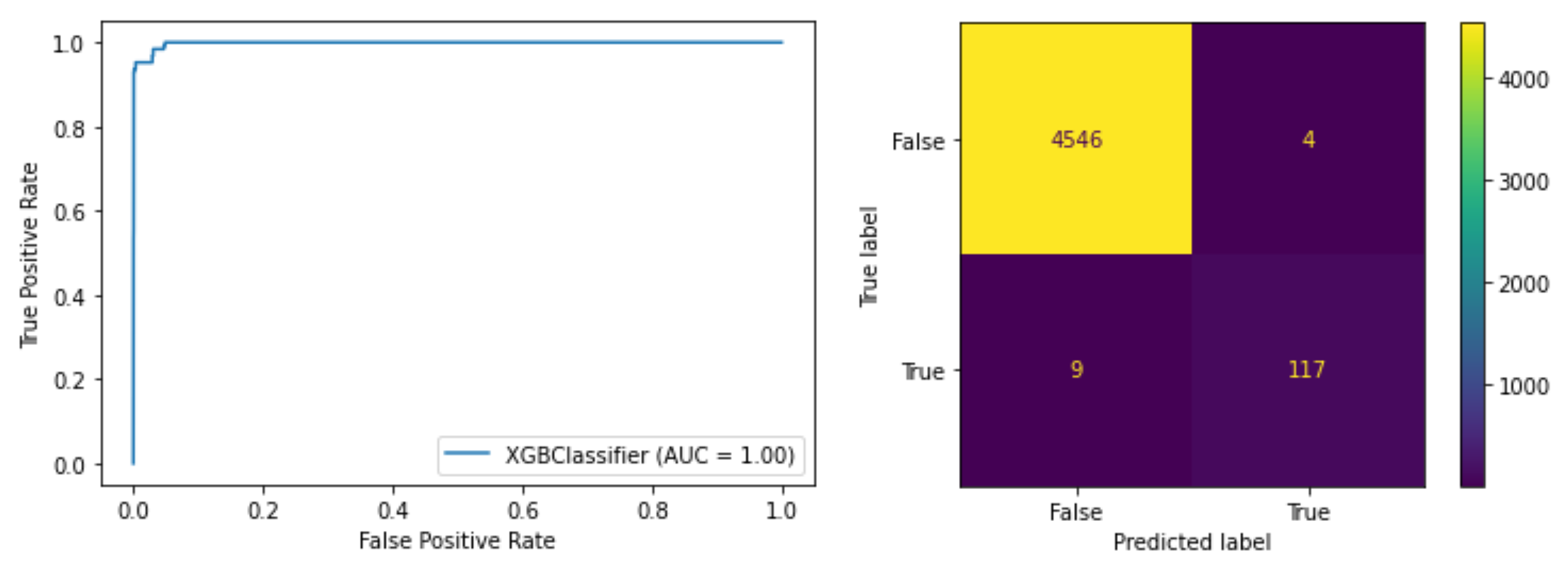
The evaluation on a test set shows that the model performs very well. It means that such model can be used in production. It’s still necessary to keep in mind that some devices might differ from the others. So it’s recommended to verify and fine tune the model on each machine before deploying it. However, model deployment is another important process that is not covered by current article.

对测试集的评估表明该模型的性能非常好。这意味着可以在生产中使用这种模型。仍然需要记住，某些设备可能与其他设备有所不同。因此，建议在部署之前在每台计算机上验证和微调模型。但是，模型部署是本文中未涉及的另一个重要过程。

To conclude, this blog post provides an example of training a model for predictive maintenance. It uses a real dataset that contains time-series telemetry values as well as information about errors and failures. The article illustrates the process of data exploration and preparation. Finally, it shows the training of Gradient Boosting model and its evaluation.

最后，这篇博客文章提供了一个培训预测性维护模型的示例。它使用包含时间序列遥测值以及有关错误和故障信息的真实数据集。本文说明了数据探索和准备的过程。最后，展示了梯度提升模型的训练及其评估。

Here you can access the notebook with original scripts.

您可以在此处使用原始脚本访问笔记本。

翻译自: https://medium.com/@andrey.i.karpov/predictive-maintenance-on-factory-data-4f8cc17696e4

预测性维护

weixin_26750511

关注

3
点赞
踩
19

收藏

觉得还不错? 一键收藏
0
评论
预测性维护_工厂数据的预测性维护

预测性维护In the era of digitization the concept of Smart Factory attracts a lot of attention. Modern industry becomes connected and highly automated. Such factories need their machines to run smoothly and...
复制链接

扫一扫