


自我监督学习和无监督学习
有关深层学习的FAU讲义 (FAU LECTURE NOTES ON DEEP LEARNING)
These are the lecture notes for FAU’s YouTube Lecture “Deep Learning”. This is a full transcript of the lecture video & matching slides. We hope, you enjoy this as much as the videos. Of course, this transcript was created with deep learning techniques largely automatically and only minor manual modifications were performed. Try it yourself! If you spot mistakes, please let us know!
这些是FAU YouTube讲座“ 深度学习 ”的 讲义 。 这是演讲视频和匹配幻灯片的完整记录。 我们希望您喜欢这些视频。 当然,此成绩单是使用深度学习技术自动创建的,并且仅进行了较小的手动修改。 自己尝试! 如果发现错误,请告诉我们!
导航 (Navigation)
Previous Lecture / Watch this Video / Top Level / Next Lecture
Welcome back to deep learning! So, today I want to talk to you about a couple of advanced topics, in particular, looking into sparse annotations. We know that data quality and annotations are extremely costly. In the next couple of videos, we want to talk about some ideas on how to save annotations. The topics will be weakly supervised learning and self-supervised learning.
欢迎回到深度学习! 因此,今天我想和您谈谈几个高级主题,尤其是研究稀疏注释。 我们知道数据质量和注释非常昂贵。 在接下来的两个视频中,我们要讨论有关如何保存注释的一些想法。 主题将是弱监督学习和自我监督学习。
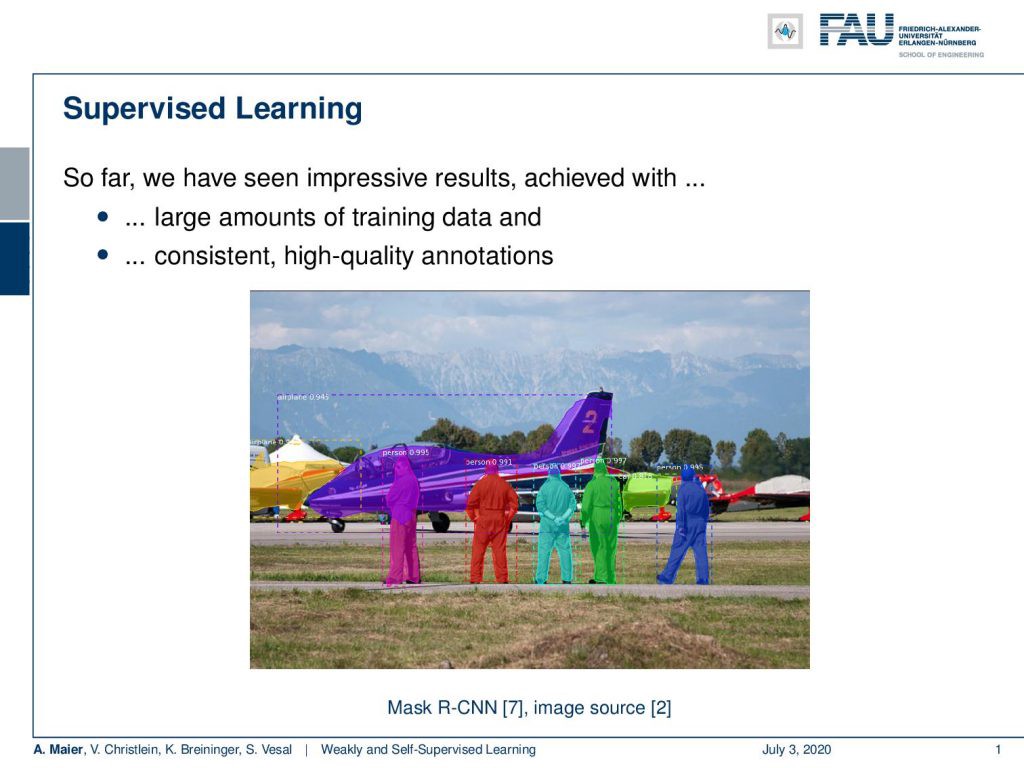
Okay. So, let’s look at our slides and see what I have for you. The topic is weakly and self-supervised learning. We start today by looking into limited annotations and some definitions. Later, we will look into self-supervised learning for representation learning. So, what’s the problem with learning with limited annotations? Well so far. we had supervised learning and we’ve seen these impressive results achieved with large amounts of training data and consistent high-quality annotations. Here, you see an example. We had annotations for instance-based segmentation and there we had simply the assumption that all of these annotations are there. We can use them and there may be even publicly available. So, it’s no big deal. But actually, in most cases, this is not true.
好的。 因此,让我们看一下幻灯片,看看我为您准备的。 主题是薄弱的自我监督学习。 我们今天从研究有限的注释和一些定义开始。 稍后,我们将研究自我监督学习,以进行表征学习。 那么,用有限的注解学习会有什么问题呢? 到目前为止。 我们对学习进行了监督,我们已经看到,通过大量的培训数据和一致的高质量注释,可以取得令人印象深刻的结果。 在这里,您将看到一个示例。 我们有基于实例的细分的注释,而我们仅假设所有这些注释都在那里。 我们可以使用它们,甚至有可能公开可用。 因此,没什么大不了的。 但是实际上,在大多数情况下,这是不正确的。
Typically, you have to annotate and annotation is very costly. If you look at image-level class labels, you will spend approximately 20 seconds per sample. So here, you can see for example the image with a dog. There are also ideas where we try to make it faster. For example by instance spotting that you can see here in [11]. If you then go to instance segmentation, you actually have to draw outlines and that’s at least 80 seconds per annotation that you have to spend here. If you go ahead to dense pixel-level annotations, you can easily spend one and a half hours for annotating an image like this one. You can see that in [4].
通常,您必须进行注释,并且注释非常昂贵。 如果查看图像级别的类标签,则每个样本将花费大约20秒。 因此,在这里,您可以看到带有狗的图像。 也有一些想法,我们试图使其更快。 例如,通过实例发现,您可以在[11]中看到。 如果您随后进行实例分割,则实际上必须绘制轮廓,并且每个注释至少要花费80秒。 如果您要进行密集的像素级注释,则可以轻松地花费一个半小时来注释这样的图像。 您可以在[4]中看到。
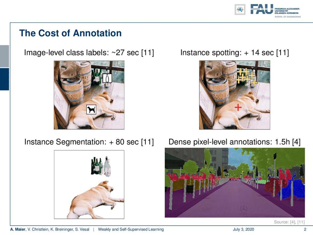
Now, the difference between weakly supervised learning and strong supervision, you can see in this graph. Here, you see that if we have image labels, of course, we can classify image labels and train. That would be essentially supervised learning: Training of bounding boxes to predict bounding boxes and training with pixel labels to predict pixel labels. Of course, you could also abstract from pixel-level labels to bounding boxes or from bounding boxes to image labels. That all would be strong supervision. Now, the idea of weakly supervised learning is that you start with image labels and go to bounding boxes, or you start with bounding boxes and try to predict pixel labels.
现在,您可以在此图中看到弱监督学习与强监督之间的区别。 在这里,您看到如果我们有图像标签,我们当然可以对图像标签进行分类和训练。 从本质上讲,这将是有监督的学习:训练边界框以预测边界框,并使用像素标签进行训练以预测像素标签。 当然,您也可以从像素级标签抽象到边界框,或者从边界框抽象到图像标签。 所有人都将受到强有力的监督。 现在,弱监督学习的思想是从图像标签开始并转到边界框,或者从边界框开始并尝试预测像素标签。
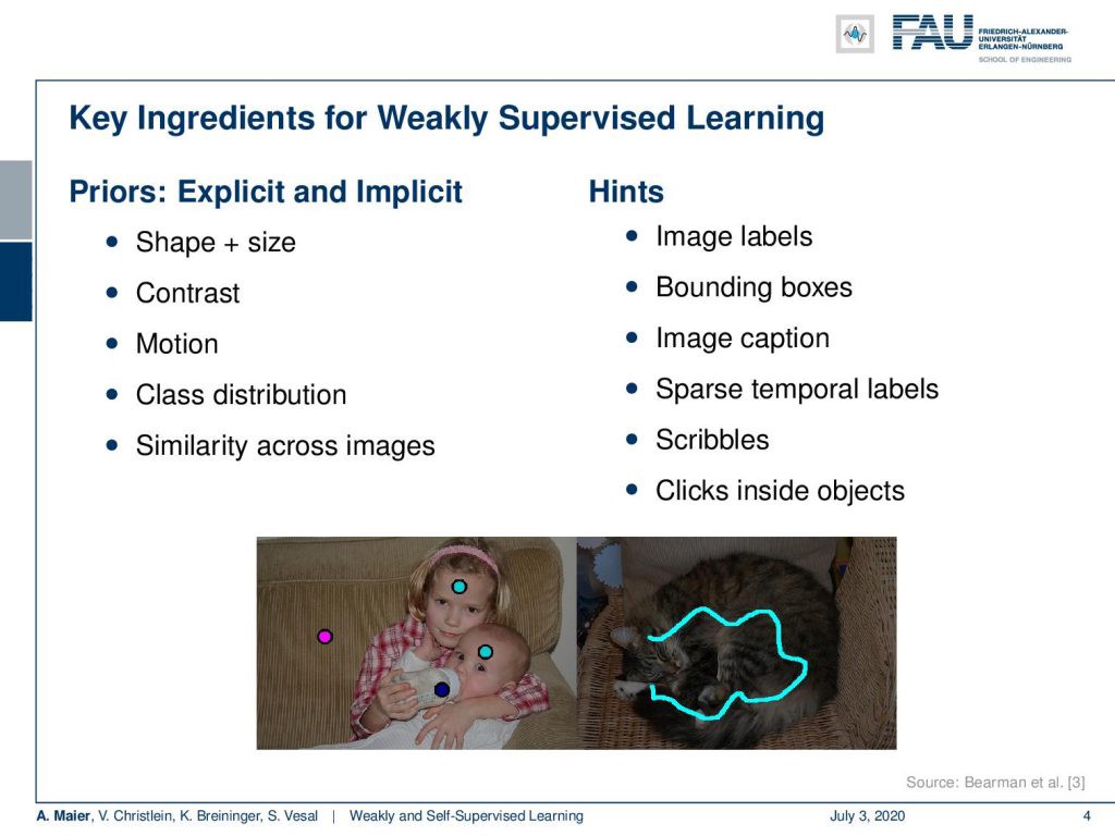
So, this is the key idea in weakly supervised learning. You somehow want to use a sparse annotation and then create much more powerful predictors. The key ingredients for weakly supervised learning are that you use priors. You use explicit and implicit priors about shape, size, and contrast. Also, motion can be used, for example, to shift bounding boxes. The class distributions tell us that some classes are much more frequent than others. Also, similarity across images helps. Of course, you can also use hints like image labels, bounding boxes, and image captions as weakly supervised labels. Sparse temporal labels are propagated over time. Scribbles or clicks inside objects are also suitable. Here, are a couple of examples of such sparse annotations for scribbles and clicks.
因此,这是弱监督学习中的关键思想。 您以某种方式想要使用稀疏注释,然后创建功能更强大的预测变量。 弱监督学习的关键因素是您使用先验知识。 您可以使用有关形状,大小和对比度的显式和隐式先验。 同样,可以使用运动来移动边界框。 班级分布告诉我们,有些班级比其他班级更频繁。 此外,图像之间的相似性也有帮助。 当然,您也可以将诸如图像标签,边框和图像标题之类的提示用作弱监督标签。 稀疏的时间标签随时间传播。 杂物或物体内部的咔嗒声也适用。 这里有几个这样的稀疏注释的示例,用于涂抹和单击。
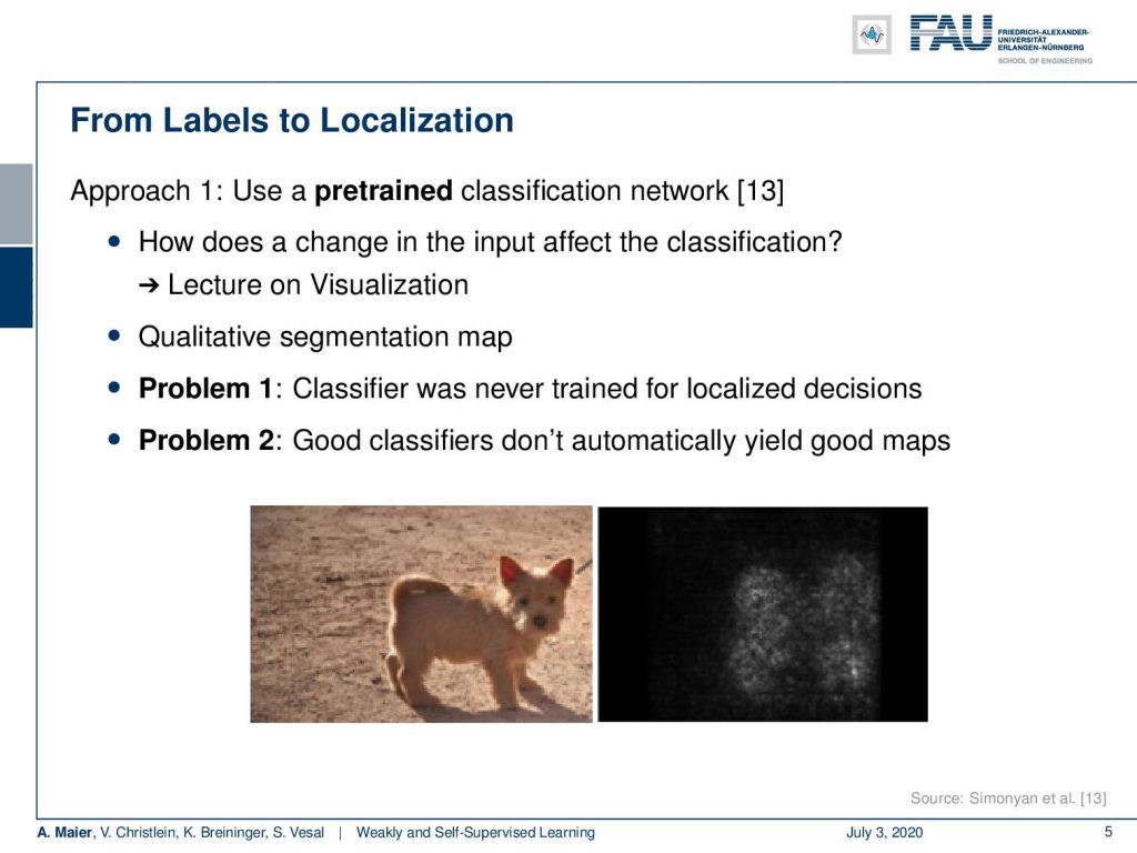
There are some general approaches. One from labels to localization would be that you use a pre-trained classification network. Then, for example, you can use tricks like in the lecture on visualization. You produce a qualitative segmentation map. So here, we had this idea of back-propagating the class label into the image domain in order to produce such labels. Now, the problem is that this classifier was never trained for localized decisions. The second problem is good classifiers don’t automatically yield good maps. So, let’s look into another idea. The key idea here is to use a global average pooling. So let’s rethink the fully convolutional networks and what we’ve been doing there.
有一些通用的方法。 从标签到本地化的一种方式是您使用预先训练的分类网络。 然后,例如,您可以使用一些技巧,例如关于可视化的讲座。 您将生成定性分割图。 因此,在这里,我们想到了将类标签反向传播到图像域中的想法,以便产生这样的标签。 现在的问题是,该分类器从未经过过本地化决策训练。 第二个问题是好的分类器不会自动产生好的地图。 因此,让我们看看另一个想法。 这里的关键思想是使用全局平均池。 因此,让我们重新考虑完全卷积网络以及我们在那里所做的事情。
You remember that we can replace fully connected layers that have only a fixed input size by M times N convolution. If you do so, we see that if we have some input image and we convolve with a tensor then essentially we get one output. Now, if we have multiple of those tensors then we would essentially get multiple channels. If we now start moving our convolution masks across the image domain, you can see that if we have a larger input image then also our outputs will grow with respect to the output domain. We’ve seen in order to resolve this, we can use global average pooling methods in order to produce the class labels per instance.
您还记得我们可以将输入大小固定为M的N卷积替换为完全连接的层。 如果这样做,我们会看到,如果我们有一些输入图像并且与张量进行卷积,则本质上我们将获得一个输出。 现在,如果我们有多个这些张量,那么我们实际上将获得多个通道。 现在,如果我们开始在图像域上移动卷积蒙版,则可以看到,如果我们有较大的输入图像,则输出也将相对于输出域增长。 我们已经看到为了解决这个问题,我们可以使用全局平均池化方法来为每个实例生成类标签。
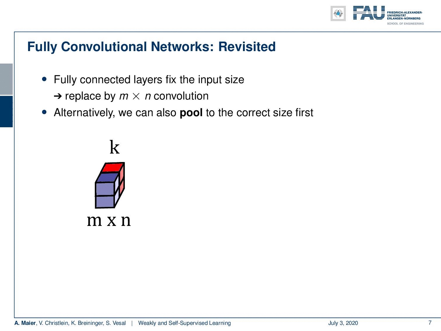
Now, what you can do also as an alternative is that you pool first to the correct size. So let’s say, this is your input then you first pool such that you can apply your classification network. Then, go to the classes in a fully connected layer. So, you essentially switch the order of the fully connected layer and the global average pooling. You global average pool first and then produce the classes. We can use this now in order to generate some labels.
现在,您还可以选择首先将池合并为正确的大小。 所以说,这是您的输入,然后您首先合并,以便可以应用分类网络。 然后,转到完全连接的层中的类。 因此,您实际上是在切换完全连接的层和全局平均池的顺序。 首先是全局平均池,然后生成类。 我们现在可以使用它来生成一些标签。
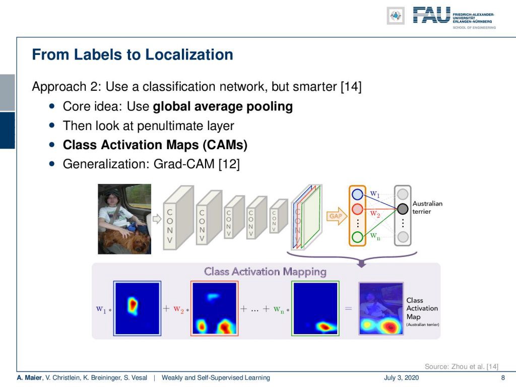
The idea is that now we look at the penultimate layer and we produce class activation maps. So, you see we have two fully connected layers that are producing the class predictions. We have essentially the input feature maps that we can an upscale to the original image size. Then, we use the weights that are assigned to the outputs of the penultimate layer, scale them accordingly, and then produce a class activation map for every output neuron. You can see that here in the bottom happening and by the way there’s also a generalization of this that is then known as Grad-CAM that you can look at in [12]. So with this, we can produce class activation maps and use that as a label for localization.
这个想法是,现在我们看倒数第二层,并生成类激活图。 因此,您看到我们有两个完全连接的层,它们在产生类预测。 本质上,我们具有输入特征图,可以将其放大到原始图像尺寸。 然后,我们使用分配给倒数第二层输出的权重,对其进行相应缩放,然后为每个输出神经元生成一个类别激活图。 您可以看到这是最底层的情况,顺便说一句,对此也有一个概括,即Grad-CAM,您可以在[12]中查看。 因此,我们可以生成类激活图并将其用作本地化的标签。
We can also go from bounding boxes to segmentation. The idea here is that we want to replace an expensively annotated, fully supervised training with bounding boxes because they’re less tedious.
我们也可以从边界框到分割。 这里的想法是,我们要用边界框代替昂贵的,带有注释的,完全受监督的培训,因为它们不太繁琐。
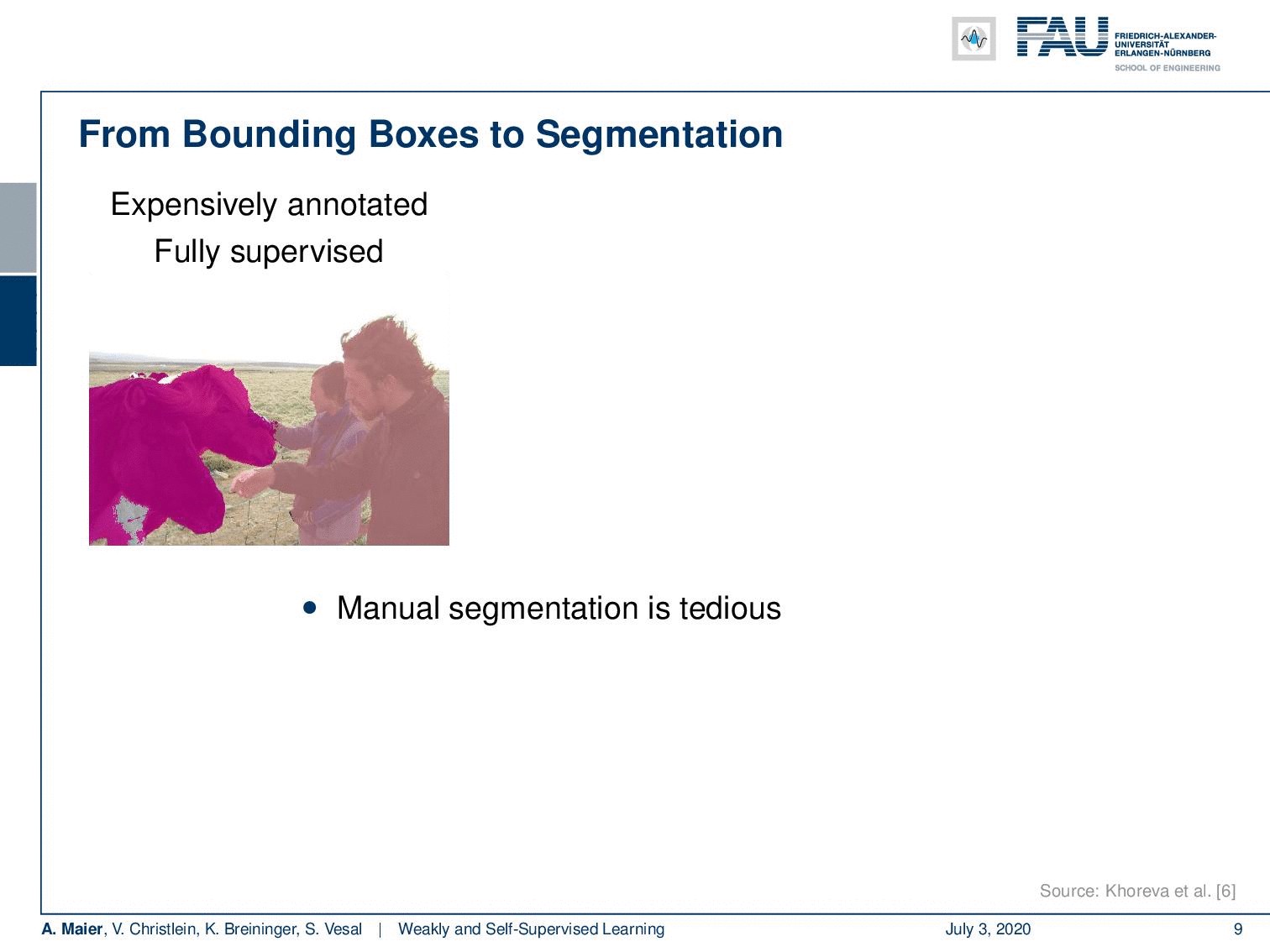
They can be annotated much quicker and of course, this results in a reduced cost. Now, the question is can we use those cheaply annotated labels and weakly supervision in order to produce good segmentations? There is actually a paper out there that looked into this idea.
可以更快地为它们添加注释,这当然可以降低成本。 现在,问题是我们是否可以使用那些带有廉价注释的标签和较弱的监管才能产生良好的细分? 实际上,有一篇论文探讨了这个想法。
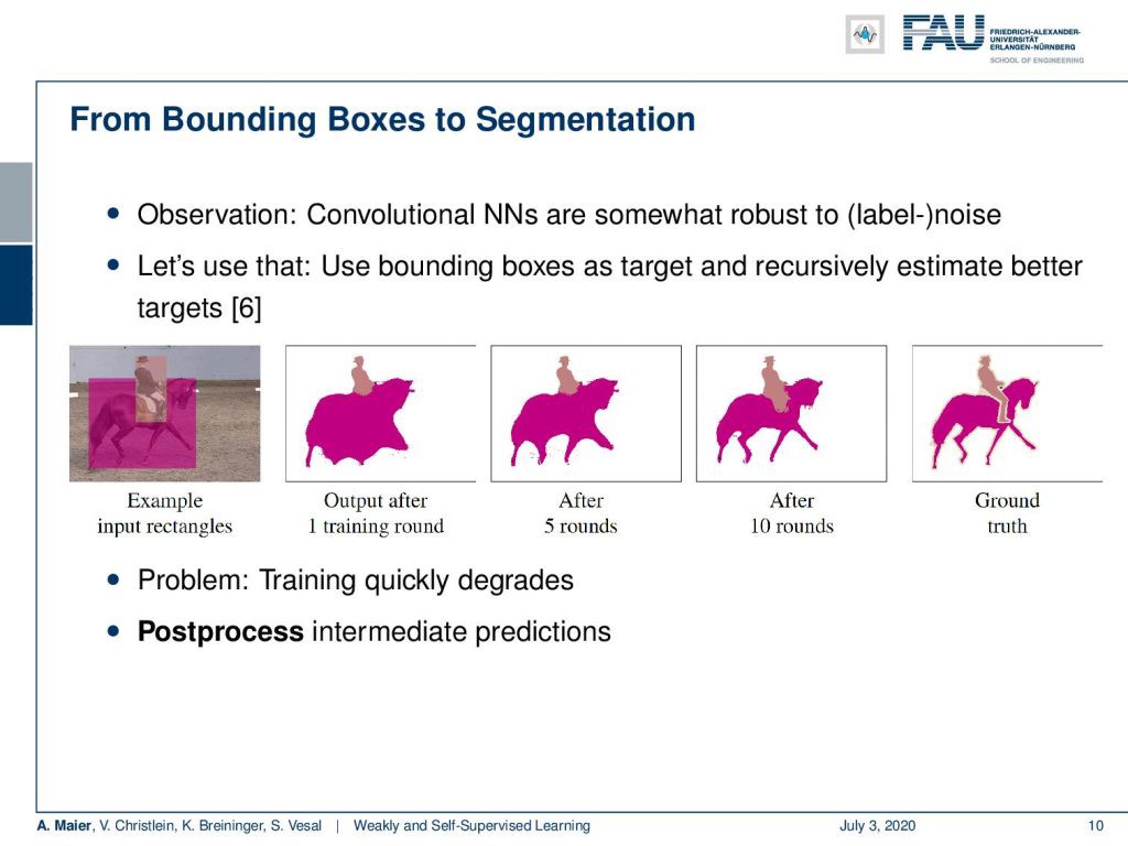
You can see that in [6]. The key idea is that you start with the input rectangles. Then, you do one round of training for a convolutional neural network. You can see that the convolutional neural network is somewhat robust to label noise and therefore if you repeat the process and refine the labels over the iterations, you can see that we get better predictions with each round of training and refining the labels. So on the right-hand side, you see the ground truth and how we gradually approach this. Now, actually there’s a problem because the training very quickly degrades. The only way how you can make this actually work is that you use post-processing in the intermediate predictions.
您可以在[6]中看到。 关键思想是从输入矩形开始。 然后,对卷积神经网络进行一轮训练。 您会看到卷积神经网络在标记噪声方面具有一定的鲁棒性,因此,如果您重复该过程并在迭代中优化标记,则可以看到,在每一轮训练和优化标记后,我们都会得到更好的预测。 因此,在右侧,您会看到基本事实以及我们如何逐步做到这一点。 现在,实际上存在一个问题,因为培训很快就会降级。 使其真正起作用的唯一方法是在中间预测中使用后处理。
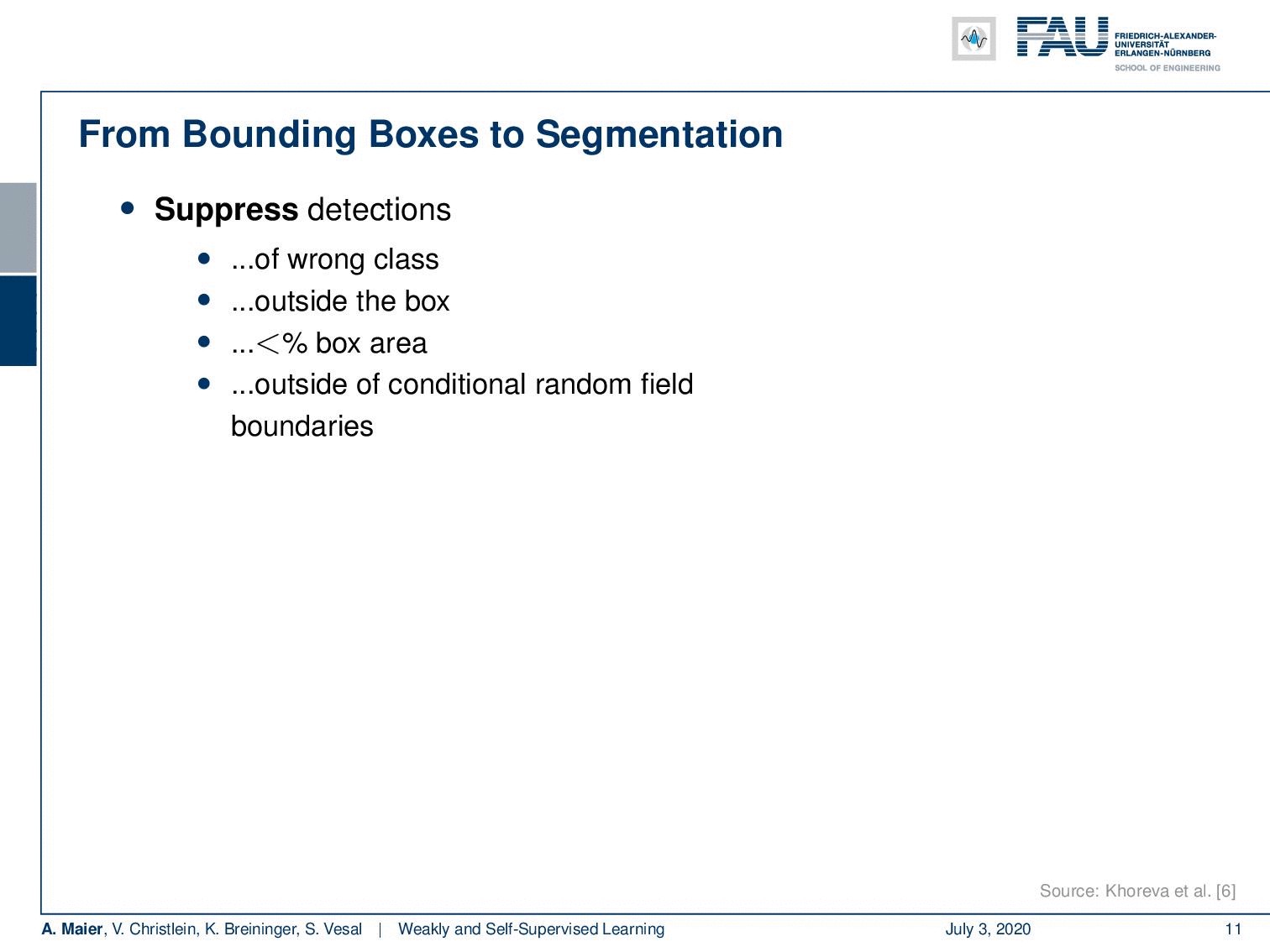
The idea that they use is that they suppress for example wrong detections. Because you have the bounding boxes, you can be sure that within that bounding box it’s unlikely to have a very different class. Then, you can also essentially remove all the predictions that are outside the bounding box. They are probably not accurate. Furthermore, you can also check if it’s less than a certain percentage of the box area, it’s probably also not an accurate label. In addition, you can use the outside of a conditional random field’s boundaries. We essentially run a kind of traditional segmentation approach to refine the boundary using edge information. You can use that as there’s no information to refine your labels. An additional improvement can be done if you use smaller boxes. On average objects are kind of roundish and therefore the corners and edges contained the least true positives. So, here are some examples of an image, and then you can define regions with unknown labels.
他们使用的想法是抑制例如错误的检测。 由于您具有边界框,因此可以确保在该边界框内不太可能具有完全不同的类。 然后,您实际上也可以删除边界框之外的所有预测。 它们可能不准确。 此外,您还可以检查它是否小于包装盒面积的一定百分比,也可能不是准确的标签。 此外,您可以使用条件随机字段边界的外部。 实际上,我们使用一种传统的分割方法来利用边缘信息来精炼边界。 您可以使用它,因为没有信息可以完善您的标签。 如果使用较小的盒子,则可以做进一步的改进。 平均而言,物体有点圆,因此拐角和边缘包含的真正值最少。 因此,这是图像的一些示例,然后您可以定义带有未知标签的区域。
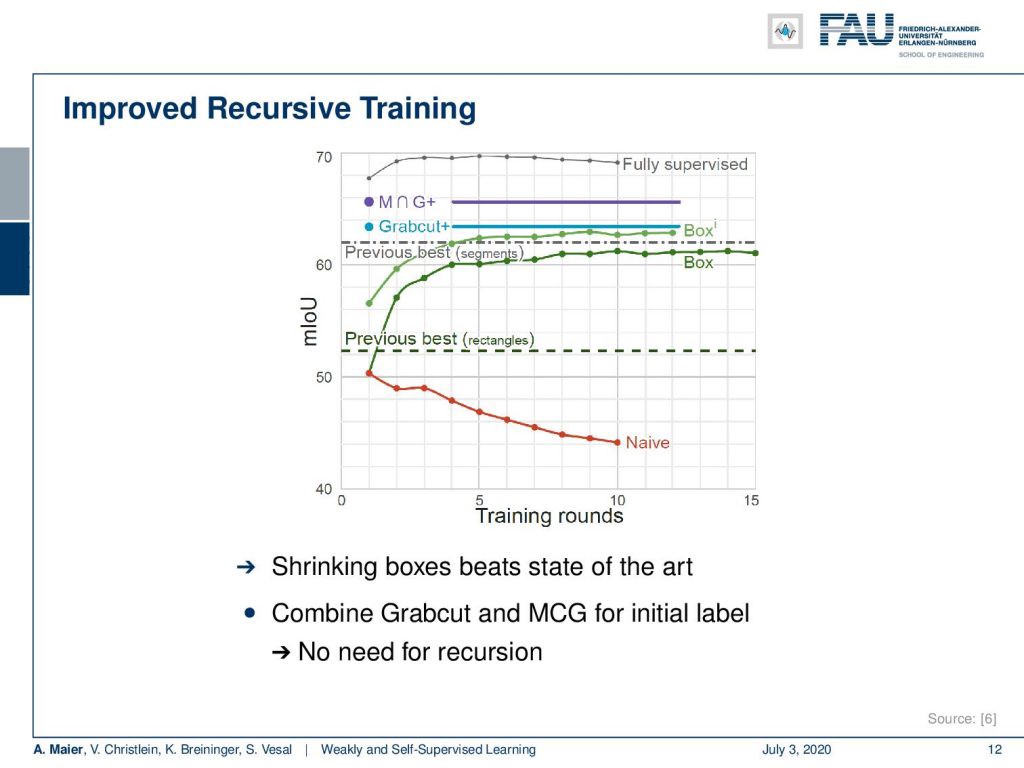
Here are some results. You can see that if we don’t do any refinement of the labels and just train the network over and over again, then you end up in this red line. In the naive approach over the number of training rounds, you actually are reducing the classification accuracy. So the network degenerates and the labels degenerate. That doesn’t work but if you use the tricks with the refinement of the labels with the boxes and excluding outliers, you can actually see that the two green curves emerge. Over the rounds of iterations, you are actually improving. To be honest, if you just use GrabCut+, then you can see that just a single round of iterations is already better than the multiple reruns of the application. If you combine GrabCut+ with the so-called MCG algorithm — the Multi-scale Combinatorial Grouping — you even end up with a better result in just one training round. So, using a heuristic method can also help to improve the labels from bounding boxes to pixel-wise labels. If you look at this, the fully supervised approach is still better. It still makes sense to do the full annotation, but we can already get pretty close in terms of performance if we use one of these weakly supervised approaches. This really depends on your target application. If you’re already ok with let’s say 65% of mean intersection over union then you might be satisfied with the weakly supervised approach. Of course, this is much cheaper than generating the very expensive ground truth annotation.
这是一些结果。 您会看到,如果我们不对标签进行任何细化,而只是一遍又一遍地训练网络,那么您最终会看到这条红线。 在幼稚的训练轮次方法中,实际上您正在降低分类准确性。 因此,网络退化,标签退化。 那是行不通的,但是如果您使用技巧来优化带有框的标签,并且排除异常值,则实际上可以看到两条绿色曲线出现了。 经过一轮迭代,您实际上正在进步。 老实说,如果您仅使用GrabCut +,那么您会发现,单轮迭代已经比应用程序的多次重新运行要好。 如果将GrabCut +与所谓的MCG算法(多尺度组合分组)相结合,甚至在一轮训练中就可以获得更好的结果。 因此,使用启发式方法还可以帮助将标签从边界框改进为逐像素标签。 如果您看一看,完全监督的方法仍然更好。 进行完整注释仍然很有意义,但是如果我们使用这些弱监督方法之一,我们在性能方面已经可以很接近了。 这实际上取决于您的目标应用程序。 如果您已经同意平均交集的65%,那么您可能会对弱监督方法感到满意。 当然,这比生成非常昂贵的地面事实注释要便宜得多。
So next time, we want to continue talking about our weakly-supervised ideas. In the next lecture, we will actually look not just into 2-D images but we’ll also look into volumes and see some smart ideas on how we can use weak annotations in order to generate volumetric 3-D segmentation algorithms. So thank you very much for listening and see you in the next lecture. Bye-bye!
因此,下一次,我们想继续谈论我们的监督薄弱的想法。 在下一讲中,我们实际上将不仅查看2-D图像,还将探究体积,并看到一些有关如何使用弱标注以生成体积3-D分割算法的精巧想法。 因此,非常感谢您的收听,并在下一堂课中再见。 再见!
If you liked this post, you can find more essays here, more educational material on Machine Learning here, or have a look at our Deep LearningLecture. I would also appreciate a follow on YouTube, Twitter, Facebook, or LinkedIn in case you want to be informed about more essays, videos, and research in the future. This article is released under the Creative Commons 4.0 Attribution License and can be reprinted and modified if referenced. If you are interested in generating transcripts from video lectures try AutoBlog.
如果你喜欢这篇文章,你可以找到这里更多的文章 ,更多的教育材料,机器学习在这里 ,或看看我们的深入 学习 讲座 。 如果您希望将来了解更多文章,视频和研究信息,也欢迎关注YouTube , Twitter , Facebook或LinkedIn 。 本文是根据知识共享4.0署名许可发布的 ,如果引用,可以重新打印和修改。 如果您对从视频讲座中生成成绩单感兴趣,请尝试使用AutoBlog 。
翻译自: https://towardsdatascience.com/weakly-and-self-supervised-learning-part-1-8d29fce2dd92
自我监督学习和无监督学习


 7412
7412


 被折叠的 条评论
为什么被折叠?
被折叠的 条评论
为什么被折叠?
 到【灌水乐园】发言


