图像去噪声卷积_卷积自动编码器可在10分钟内减少图像噪声

最新推荐文章于 2023-05-05 11:30:43 发布

weixin_26756255

最新推荐文章于 2023-05-05 11:30:43 发布

阅读量1.1k

点赞数

文章标签：卷积计算机视觉 python opencv 卷积神经网络

原文链接：https://towardsdatascience.com/image-noise-reduction-in-10-minutes-with-convolutional-autoencoders-d16219d2956a

版权

图像去噪声卷积

If you are reading this article, I am sure that we share similar interests and are/will be in similar industries. So let’s connect via Linkedin! Please do not hesitate to send a contact request! Orhan G. Yalçın — Linkedin

如果您正在阅读本文，我相信我们拥有相似的兴趣并且将会/将会从事相似的行业。 因此，让我们通过 Linkedin 连接！ 请不要犹豫，发送联系请求！ Orhan G.Yalçın— Linkedin

If you are on this page, you are also probably somewhat familiar with different neural network architectures. You have probably heard of feedforward neural networks, CNNs, RNNs and that these neural networks are very good for solving supervised learning tasks such as regression and classification.

如果您在此页面上，则可能还对不同的神经网络体系结构有些熟悉。 您可能听说过前馈神经网络，CNN，RNN，并且这些神经网络非常适合解决监督学习任务，例如回归和分类。

But, we have a whole world of problems on the unsupervised learning sphere such as dimensionality reduction, feature extraction, anomaly detection, data generation, and augmentation as well as noise reduction. For these tasks, we need the help of special neural networks that are developed particularly for unsupervised learning tasks. Therefore, they must be able to solve mathematical equations without needing supervision. One of these special neural network architectures is autoencoders.

但是，在无人监督的学习领域中，我们面临着很多问题，例如降维，特征提取，异常检测，数据生成，增强和降噪。 对于这些任务，我们需要专门为无监督学习任务而开发的特殊神经网络的帮助。 因此，他们必须能够在不需要监督的情况下求解数学方程。 这些特殊的神经网络体系结构之一就是自动编码器 。

演示地址

Get the Latest Machine Learning Tutorials

获取最新的机器学习教程

自动编码器 (Autoencoders)

什么是自动编码器？ (What are autoencoders?)

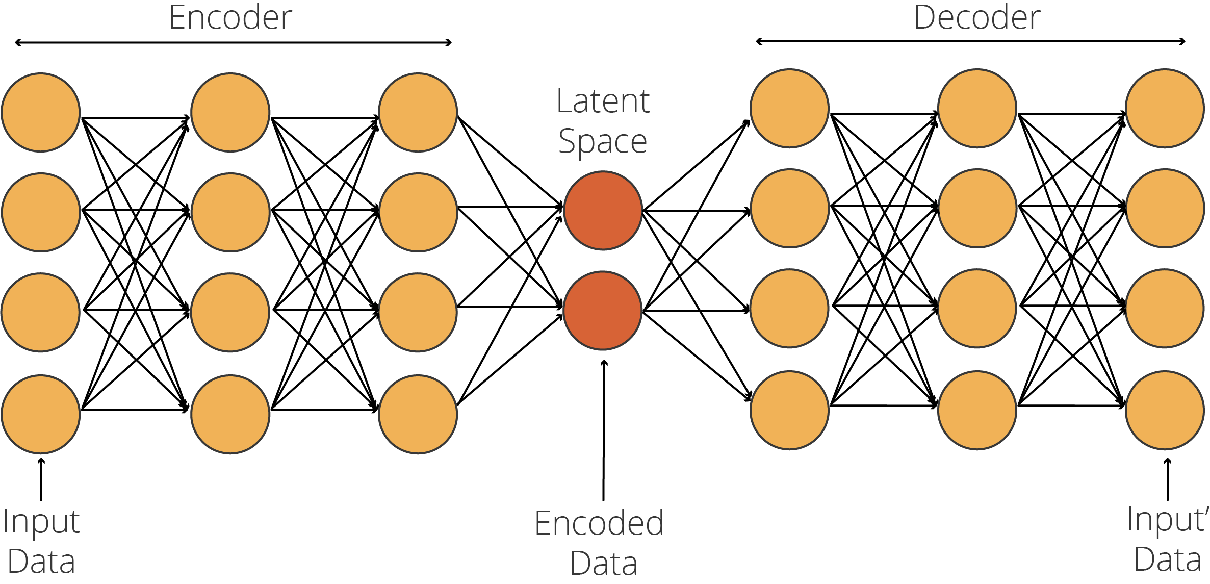
Autoencoders are neural network architectures that consist of two sub-networks, namely, encoder and decoder networks, which are tied to each other with a latent space. Autoencoders were first developed by Geoffrey Hinton, one of the most respected scientists in the AI community, and the PDP group in the 1980s. Hinton and the PDP Group aimed to address the “backpropagation without a teacher” problem, a.k.a. unsupervised learning, by using the input as the teacher. In other words, they simply used feature data both as feature data and label data. Let’s take a closer look at how autoencoders work!

自动编码器是一种神经网络体系结构，由两个子网络组成，即编码器网络和解码器网络，它们之间相互关联并具有潜在的空间。自动编码器最早由AI社区中最受尊敬的科学家之一Geoffrey Hinton和1980年代的PDP组开发。 Hinton和PDP集团旨在通过使用输入内容作为老师来解决“无师自传”问题，也就是无监督学习。换句话说，他们只是简单地将要素数据用作要素数据和标签数据。让我们仔细看看自动编码器的工作原理！

Image for post — Figure 2. An Autoencoder Network with Encoder and Decoder Networks

自动编码器架构 (Autoencoder Architecture)

Autoencoders consists of an encoder network, which takes the feature data and encodes it to fit into the latent space. This encoded data (i.e., code) is used by the decoder to convert back to the feature data. In an encoder, what the model learns is how to encode the data efficiently so that the decoder can convert it back to the original. Therefore, the essential part of autoencoder training is to generate an optimized latent space.

自动编码器由一个编码器网络组成，该网络获取特征数据并将其编码以适合潜在空间。解码器使用此编码数据(即代码)将其转换回特征数据。在编码器中，模型学习的是如何有效地对数据进行编码，以便解码器可以将其转换回原始数据。因此，自动编码器训练的必要部分是生成优化的潜在空间。

Now, know that in most cases, the number of neurons in the latent space is much smaller than the input and output layers, but it does not have to be that way. There are different types of autoencoders such as undercomplete, overcomplete, sparse, denoising, contractive, and variational autoencoders. In this tutorial, we only focus on undercomplete autoencoders which are used for denoising.

现在，知道在大多数情况下，潜伏空间中神经元的数量要比输入和输出层小得多，但这不是必须的。有多种类型的自动编码器，例如不完全，过度完成，稀疏，去噪，压缩和变体自动编码器。在本教程中，我们仅关注用于降噪的不完整自动编码器。

自动编码器中的图层 (Layers in an Autoencoder)

The standard practice when building an autoencoder is to design an encoder and to create an inversed version of this network as the decoder of this autoencoder. So, as long as there is an inverse relationship between the encoder and the decoder network, you are free to add any layer to these sub-networks. For example, if you are dealing with image data, you would surely need convolution and pooling layers. On the other hand, if you are dealing with sequence data, you would probably need LSTM, GRU, or RNN units. The important point here is that you are free to build anything you want.

构建自动编码器时的标准做法是设计一个编码器，并创建该网络的反向版本作为该自动编码器的解码器。因此，只要编码器和解码器网络之间存在反比关系，您就可以随意在这些子网中添加任何层。例如，如果要处理图像数据，则肯定需要卷积层和池化层。另一方面，如果要处理序列数据，则可能需要LSTM，GRU或RNN单元。这里的重点是您可以自由构建所需的任何东西。

And now that you have an idea of autoencoders that you can build for image noise reduction, we can move on to the tutorial and start writing our code for our image noise reduction model. For the tutorial, we choose to do our own take on one of TensorFlow’s official tutorials, Intro to Autoencoders [1] and we will use a very popular dataset among the members of the AI community: Fashion MNIST.

现在，您有了可以构建的用于减少图像噪声的自动编码器的概念，我们可以继续学习本教程，并开始为图像噪声降低模型编写代码。对于本教程，我们选择自己使用TensorFlow的官方教程之一，即Autoencoders简介[1] ，我们将使用AI社区成员中非常流行的数据集： Fashion MNIST 。

下载时尚MNIST数据集 (Downloading the Fashion MNIST Dataset)

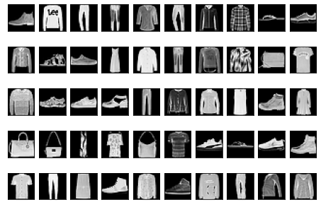
Fashion-MNIST is designed and maintained by Zalando, a European e-commerce company based in Berlin, Germany. Fashion MNIST consists of a training set of 60,000 images and a test set of 10,000 images. Each example is a 28×28 grayscale image, associated with a label from 10 classes. Fashion MNIST, which contains images of clothing items (as shown in Figure 4), is designed as an alternative dataset to the MNIST dataset, which contains handwritten digits. We choose Fashion MNIST simply because MNIST is already overused in many tutorials.

Fashion-MNIST由位于德国柏林的欧洲电子商务公司Zalando设计和维护。 Fashion MNIST包含60,000张图像的训练集和10,000张图像的测试集。每个示例都是一个28×28灰度图像，与来自10个类别的标签关联。 Fashion MNIST包含服装的图像(如图4所示)，被设计为MNIST数据集的替代数据集，该数据集包含手写数字。我们之所以选择Fashion MNIST，仅仅是因为MNIST已在许多教程中被过度使用。

The lines below import TensorFlow and load Fashion MNIST:

下面的行导入TensorFlow并加载Fashion MNIST：

import tensorflow as tf
from tensorflow.keras.datasets import fashion_mnist
# We don't need y_train and y_test
(x_train, _), (x_test, _) = fashion_mnist.load_data()
print('Max value in the x_train is', x_train[0].max())
print('Min value in the x_train is', x_train[0].min())

Now let’s generate a grid with samples from our dataset with the following lines:

现在，让我们使用来自以下行的数据集样本生成一个网格：

import matplotlib.pyplot as plt


fig, axs = plt.subplots(5, 10) 
fig.tight_layout(pad=-1)
plt.gray()
a = 0 
for i in range(5): 
  for j in range(10): 
    axs[i, j].imshow(tf.squeeze(x_test[a])) 
    axs[i, j].xaxis.set_visible(False) 
    axs[i, j].yaxis.set_visible(False) 
    a = a + 1

Our output shows the first 50 samples from the test dataset:

我们的输出显示了测试数据集中的前50个样本：

处理时尚MNIST数据 (Processing the Fashion MNIST Data)

For computational efficiency and model reliability, we have to apply Minmax normalization to our image data, limiting the value range between 0 and 1. Since our data is in RGB format, the minimum value is 0 and the maximum value is 255 and we can conduct the Minmax normalization operation with the following lines:

为了提高计算效率和模型可靠性，我们必须对图像数据应用Minmax归一化，将值范围限制在0到1之间。由于我们的数据是RGB格式，因此最小值为0，最大值为255，我们可以进行使用以下几行的Minmax规范化操作：

x_train = x_train.astype('float32') / 255.
x_test = x_test.astype('float32') / 255.

We also have to reshape our NumPy array as the current shape of the datasets is (60000, 28, 28) and (10000, 28, 28). We just need to add a fourth dimension with a single value (e.g., from (60000, 28, 28) to (60000, 28, 28, 1)). The fourth dimension acts pretty much as proof that our data is in grayscale format with a single value representing color information ranging from white to black. If we’d have colored images, then we would need three values in our fourth dimension. But all we need is a fourth dimension containing a single value since we use grayscale images. The following lines do this:

我们还必须重塑NumPy数组，因为数据集的当前形状是(60000，28，28)和(10000，28，28)。我们只需要添加一个具有单个值的第四维(例如，从(60000，28，28)到(60000，28，28，1))。第四维几乎可以证明我们的数据是灰度格式，其中一个值代表从白色到黑色的颜色信息。如果我们要彩色图像，则在第四维中需要三个值。但是我们只需要包含单个值的第四维，因为我们使用灰度图像。以下几行执行此操作：

x_train = x_train[…, tf.newaxis]
x_test = x_test[…, tf.newaxis]

Let’s take a look at the shape of our NumPy arrays with the following lines:

让我们用以下几行来看看我们的NumPy数组的形状：

print(x_train.shape)
print(x_test.shape)

Output: (60000, 28, 28, 1) and (10000, 28, 28, 1)

输出： (60000，28，28，1)和(10000，28，28，1)

给图像添加噪点 (Adding Noise to the Images)

Remember our goal is to build a model, which is capable of performing noise reduction on images. To be able to do this, we will use existing image data and add them to random noise. Then, we will feed the original images as input and noisy images as output. Our autoencoder will learn the relationship between a clean image and a noisy image and how to clean a noisy image. So let’s create a noisy version of our Fashion MNIST dataset.

请记住，我们的目标是建立一个模型，该模型能够对图像进行降噪。为此，我们将使用现有的图像数据并将其添加到随机噪声中。然后，我们将原始图像作为输入，将嘈杂图像作为输出。我们的自动编码器将学习干净图像和噪点图像之间的关系以及如何清理噪点图像。因此，让我们为我们的Fashion MNIST数据集创建一个嘈杂的版本。

For this task, we add a randomly generated value to each array item by using tf.random.normal method. Then, we multiply the random value with a noise_factor, which you can play around with. The following code adds noise to images:

对于此任务，我们使用tf.random.normal方法将随机生成的值添加到每个数组项。然后，我们将随机值与noise_factor相乘，您可以使用它。以下代码会增加图像的噪点：

noise_factor = 0.4
x_train_noisy = x_train + noise_factor * tf.random.normal(shape=x_train.shape) 
x_test_noisy = x_test + noise_factor * tf.random.normal(shape=x_test.shape)

We also need to make sure that our array item values are within the range of 0 to 1. For this, we may use tf.clip_by_value method. clip_by_value is a TensorFlow method which clips the values outside of the Min-Max range and replaces them with the designated min or max value. The following code clips the values out of range:

我们还需要确保数组项的值在0到1的范围内。为此，我们可以使用tf.clip_by_value方法。 clip_by_value是TensorFlow方法，可将值裁剪到Min-Max范围之外，并将其替换为指定的min或max值。以下代码将值裁剪为超出范围：

x_train_noisy = tf.clip_by_value(x_train_noisy, clip_value_min=0., clip_value_max=1.) 
x_test_noisy = tf.clip_by_value(x_test_noisy, clip_value_min=0., clip_value_max=1.)

Now that we created a regularized and noisy version of our dataset, we can check out how it looks:

现在，我们创建了数据集的正则化和嘈杂版本，我们可以检查一下它的外观：

n = 5
plt.figure(figsize=(20, 8))
plt.gray()
for i in range(n):
  ax = plt.subplot(2, n, i + 1) 
  plt.title("original", size=20) 
  plt.imshow(tf.squeeze(x_test[i])) 
  plt.gray() 
  bx = plt.subplot(2, n, n+ i + 1) 
  plt.title("original + noise", size=20) 
  plt.imshow(tf.squeeze(x_test_noisy[i])) 
plt.show()

As you can see, it is almost impossible to understand what we see in noisy images. However, our autoencoders will marvelously learn to clean it.

如您所见，几乎不可能理解我们在嘈杂图像中看到的内容。但是，我们的自动编码器将非常学习如何清洁它。

建立我们的模型 (Building Our Model)

In TensorFlow, apart from Sequential API and Functional API, there is a third option to build models: Model subclassing. In model subclassing, we are free to implement everything from scratch. Model subclassing is fully customizable and enables us to implement our own custom model. It is a very powerful method since we can build any type of model. However, it requires a basic level of object-oriented programming knowledge. Our custom class would subclass the tf.keras.Model object. It also requires declaring several variables and functions. However, it is nothing to be afraid of.

在TensorFlow中，除了顺序API和功能性API外，还有第三个选项来构建模型：模型子类化。在模型子类化中，我们可以自由地从头开始实现所有功能。模型子类是完全可定制的，并使我们能够实现自己的定制模型。这是一种非常强大的方法，因为我们可以构建任何类型的模型。但是，它需要基本水平的面向对象编程知识。我们的自定义类将把tf.keras.Model对象作为子类。它还需要声明几个变量和函数。但是，不用担心。

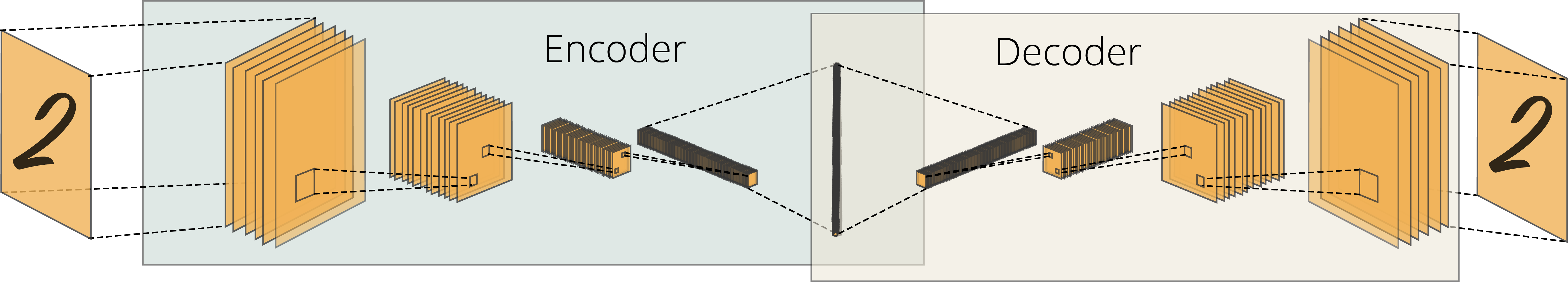
Also note that since we are dealing with image data, it is more efficient to build a convolutional autoencoder, which would look like this:

还要注意，由于我们正在处理图像数据，因此构建卷积自动编码器的效率更高，如下所示：

To build a model, we simply need to complete the following tasks:

要构建模型，我们只需要完成以下任务：

Create a class extending the keras.Model object
创建一个扩展keras.Model对象的类
Create an __init__ function to declare two separate models built with Sequential API. Within them, we need to declare layers that would reverse each other. One Conv2D layer for the encoder model whereas one Conv2DTranspose layer for the decoder model.
创建一个__init__函数来声明使用Sequential API构建的两个单独的模型。在它们内部，我们需要声明可以相互反转的层。一层Conv2D层用于编码器模型，一层Conv2DTranspose层用于解码器模型。
Create a call function to tell the model how to process the inputs using the initialized variables with __init__ method:
创建一个调用函数来告诉模型如何使用带有__init__方法的初始化变量来处理输入：
We need to call the initialized encoder model which takes the images as input
我们需要调用初始化的编码器模型，该模型将图像作为输入
We also need to call the initialized decoder model which takes the output of the encoder model (encoded) as input
我们还需要调用初始化的解码器模型，该模型将编码器模型的输出(已编码)作为输入
Return the output of the decoder
返回解码器的输出

We can achieve all of them with the code below:

我们可以使用以下代码实现所有这些目标：

from tensorflow.keras.layers import Conv2DTranspose, Conv2D, Input


class NoiseReducer(tf.keras.Model): 
  def __init__(self):


    super(NoiseReducer, self).__init__() 


    self.encoder = tf.keras.Sequential([ 
      Input(shape=(28, 28, 1)), 
      Conv2D(16, (3,3), activation='relu', padding='same', strides=2), 
      Conv2D(8, (3,3), activation='relu', padding='same', strides=2)]) 
    
    self.decoder = tf.keras.Sequential([ 
      Conv2DTranspose(8, kernel_size=3, strides=2, activation='relu', padding='same'), 
      Conv2DTranspose(16, kernel_size=3, strides=2, activation='relu', padding='same'), 
      Conv2D(1, kernel_size=(3,3), activation='sigmoid', padding='same')]) 
  
  def call(self, x): 
    encoded = self.encoder(x) 
    decoded = self.decoder(encoded) 
    return decoded

And let’s create the model with an object call:

让我们通过对象调用创建模型：

autoencoder = NoiseReducer()

配置我们的模型 (Configuring Our Model)

For this task, we will use an Adam optimizer and Mean Squared Error for our model. We can easily use <strong>compile</strong> function to configure our autoencoder, as shown below:

对于此任务，我们将为模型使用Adam优化器和均方误差。我们可以轻松地使用<strong> compile </ strong>函数来配置我们的自动编码器，如下所示：

autoencoder.compile(optimizer='adam', loss='mse')

Finally, we can run our model for 10 epochs by feeding the noisy and the clean images, which will take about 1 minute to train. We also use test datasets for validation. The following code is for training the model:

最后，我们可以通过输入噪声和干净的图像来运行模型10个纪元，这大约需要1分钟的训练时间。我们还使用测试数据集进行验证。以下代码用于训练模型：

autoencoder.fit(x_train_noisy, 
                x_train, 
                epochs=10, 
                shuffle=True, 
                validation_data=(x_test_noisy, x_test))

使用我们训练有素的自动编码器降低图像噪声 (Reducing Image Noise with Our Trained Autoencoder)

Now that we trained our autoencoder, we can start cleaning noisy images. Note that we have access to both encoder and decoder networks since we define them under the NoiseReducer object.

既然我们已经训练了自动编码器，我们就可以开始清除噪点图像。请注意，由于我们在NoiseReducer对象下定义它们，因此我们可以访问编码器和解码器网络。

So, first, we will use an encoder to encode our noisy test dataset (x_test_noisy). Then, we will take the encoded output from the encoder to feed into the decoder to obtain the cleaned image. The following lines complete these tasks:

因此，首先，我们将使用编码器对嘈杂的测试数据集(x_test_noisy)进行编码。然后，我们将从编码器获取编码后的输出以馈入解码器以获得清洁后的图像。以下行完成了这些任务：

encoded_imgs=autoencoder.encoder(x_test_noisy).numpy()
decoded_imgs=autoencoder.decoder(encoded_imgs)

and let’s plot the first 10 samples for a side-by-side comparison:

让我们绘制前10个样本以进行并排比较：

n = 10 
plt.figure(figsize=(20, 7))
plt.gray()
for i in range(n): 
  # display original + noise 
  bx = plt.subplot(3, n, i + 1) 
  plt.title("original + noise") 
  plt.imshow(tf.squeeze(x_test_noisy[i])) 
  ax.get_xaxis().set_visible(False) 
  ax.get_yaxis().set_visible(False) 
  
  # display reconstruction 
  cx = plt.subplot(3, n, i + n + 1) 
  plt.title("reconstructed") 
  plt.imshow(tf.squeeze(decoded_imgs[i])) 
  bx.get_xaxis().set_visible(False) 
  bx.get_yaxis().set_visible(False) 
  
  # display original 
  ax = plt.subplot(3, n, i + 2*n + 1) 
  plt.title("original") 
  plt.imshow(tf.squeeze(x_test[i])) 
  ax.get_xaxis().set_visible(False) 
  ax.get_yaxis().set_visible(False) 


plt.show()

The first row is for noisy images, the second row is for cleaned (reconstructed) images, and finally, the third row is for original images. See how the cleaned images are similar to the original images:

第一行用于嘈杂的图像，第二行用于清洁(重建)的图像，最后第三行用于原始图像。查看清理后的图像与原始图像的相似之处：

恭喜啦 (Congratulations)

You have built an autoencoder model, which can successfully clean very noisy images, which it has never seen before (we used the test dataset). There are obviously some non-recovered distortions, such as the missing bottom of the slippers in the second image from the right. Yet, if you consider how deformed the noisy images, we can say that our model is pretty successful in recovering the distorted images.

您已经建立了一个自动编码器模型，该模型可以成功清除非常嘈杂的图像，这是以前从未见过的( 我们使用了测试数据集 )。显然存在一些无法恢复的失真，例如右图第二张图像中拖鞋的底部丢失。但是，如果考虑带噪图像的变形程度，可以说我们的模型在恢复失真图像方面非常成功。

Off the top of my head, you can -for instance- consider extending this autoencoder and embed it into a photo enhancement app, which can increase the clarity and crispiness of the photos.

例如，您可以考虑扩展此自动编码器并将其嵌入到照片增强应用程序中，这可以提高照片的清晰度和清晰度。