Caffe第一个例子

最新推荐文章于 2021-03-18 00:59:31 发布

weixin_34043301

最新推荐文章于 2021-03-18 00:59:31 发布

阅读量65

点赞数

文章标签：人工智能 python

原文链接：https://my.oschina.net/propagator/blog/1031499

版权

2019独角兽企业重金招聘Python工程师标准>>>

安装好caffe之后，可以尝试下caffe自带的例子mnist。官方教程如下：

http://caffe.berkeleyvision.org/gathered/examples/mnist.html

首先运行如下命令，下载MNIST数据

cd $CAFFE_ROOT
./data/mnist/get_mnist.sh
./examples/mnist/create_mnist.sh

其中$CAFFE_ROOT代表安装caffe的目录。但是很可能无法下载，因为要求安装wget和gunzip，而windows下wget和gunzip需要另行安装。因此可查看get_mnist.sh文件，手动下载如下四个文件

http://yann.lecun.com/exdb/mnist/train-images-idx3-ubyte.gz

http://yann.lecun.com/exdb/mnist/train-labels-idx1-ubyte.gz

http://yann.lecun.com/exdb/mnist/t10k-images-idx3-ubyte.gz

http://yann.lecun.com/exdb/mnist/t10k-labels-idx1-ubyte.gz

下载之后解压到$CAFFE_ROOT/data/mnist/文件夹下。如下图所示

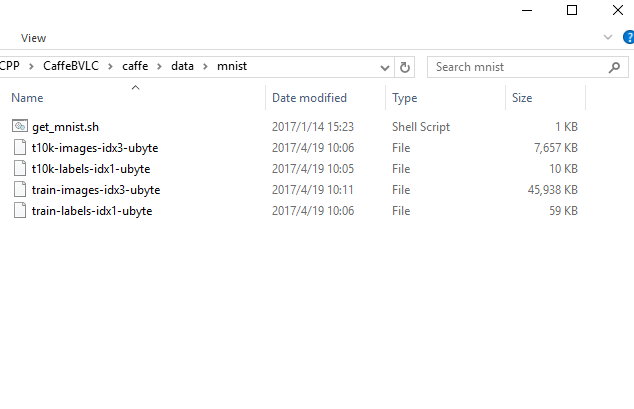
此处CaffeBVLC\caffe目录即为$CAFFE_ROOT。

接下来将$CAFFE_ROOT\build\examples\mnist\Release\convert_mnist_data.exe复制到$CAFFE_ROOT\examples\mnist\目录下，并执行如下指令

cd $CAFFE_ROOT\examples\mnist
convert_mnist_data.exe ..\..\data\mnist\train-images-idx3-ubyte \
  ..\..\data\mnist\train-labels-idx1-ubyte mnist_train_lmdb --backend=lmdb
convert_mnist_data.exe ..\..\data\mnist\t10k-images-idx3-ubyte \
  ..\..\data\mnist\t10k-labels-idx1-ubyte mnist_test_lmdb --backend=lmdb

注意执行过程中可能遇到缺少dll的报错，把所有缺少的dll都从$CAFFE_ROOT目录中找到，然后复制到$CAFFE_ROOT\examples\mnist目录中即可，如下图所示（python27.dll需从python安装目录处获得；或者在Anaconda的python2.7终端中运行，则无需复制python27.dll。以下命令皆为在Anaconda环境中执行）

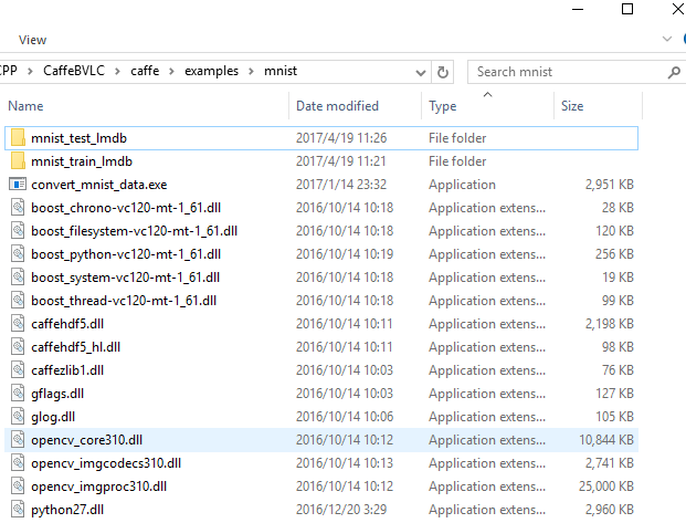
执行上述指令后，该目录下多了两个目录，mnist_test_lmdb和mnist_train_lmdb，如上图所示。

将之前可以成功运行的caffe.exe所在目录添加到PATH环境变量中，该目录为$CAFFE_ROOT\build\tools\Release，然后在$CAFFE_ROOT目录下运行如下命令（此处可参考上一篇文章《Windows下安装TensorFlow和Caffe》）

cd $CAFFE_ROOT
caffe.exe train --solver=examples\mnist\lenet_solver.prototxt

运行结果如下

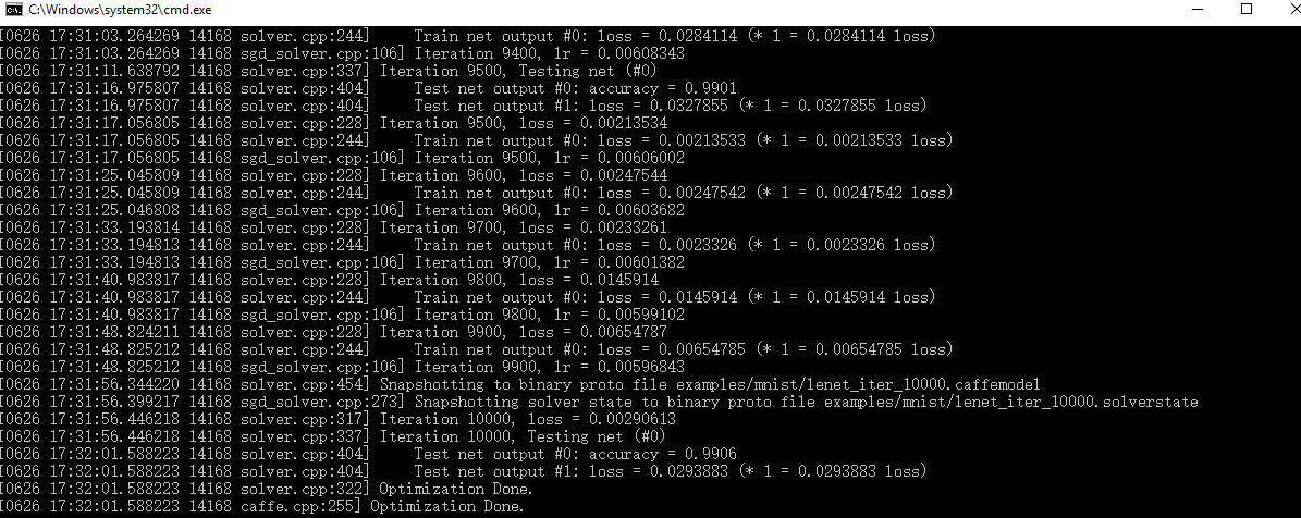
上图的输出表明，caffe成功运行，对mnist数据集进行了训练和测试。训练模型保存在$CAFFE_ROOT\examples\mnist\lenet_iter_10000.caffemodel文件中，可部署在应用中进行识别。

下面简单介绍一下caffe中的模型定义和配置文件。首先看看lenet_solver.prototxt，其内容如下

# The train/test net protocol buffer definition
net: "examples/mnist/lenet_train_test.prototxt"
# test_iter specifies how many forward passes the test should carry out.
# In the case of MNIST, we have test batch size 100 and 100 test iterations,
# covering the full 10,000 testing images.
test_iter: 100
# Carry out testing every 500 training iterations.
test_interval: 500
# The base learning rate, momentum and the weight decay of the network.
base_lr: 0.01
momentum: 0.9
weight_decay: 0.0005
# The learning rate policy
lr_policy: "inv"
gamma: 0.0001
power: 0.75
# Display every 100 iterations
display: 100
# The maximum number of iterations
max_iter: 10000
# snapshot intermediate results
snapshot: 5000
snapshot_prefix: "examples/mnist/lenet"
# solver mode: CPU or GPU
solver_mode: CPU

第一行定义了模型文件的位置，后面两行定义了测试迭代次数，迭代100次，每500次训练进行一次网络测试。base_lr，momentum和weight_decay定义了网络学习速率，动量和权重衰减速率。lr_policy，gamma和power定义了优化算法及参数，display定义了每100次迭代显示一次结果，max_iter定义了最大迭代次数。snapshot和snapshot_prefix定义了每隔多少次训练保存一次网络参数，以及网络参数保存的文件前缀（包括目录）。solver_mode定义了CPU计算还是GPU计算。

然后看看lenet_train_test.prototxt

name: "LeNet"
layer {
  name: "mnist"
  type: "Data"
  top: "data"
  top: "label"
  include {
    phase: TRAIN
  }
  transform_param {
    scale: 0.00390625
  }
  data_param {
    source: "examples/mnist/mnist_train_lmdb"
    batch_size: 64
    backend: LMDB
  }
}
layer {
  name: "mnist"
  type: "Data"
  top: "data"
  top: "label"
  include {
    phase: TEST
  }
  transform_param {
    scale: 0.00390625
  }
  data_param {
    source: "examples/mnist/mnist_test_lmdb"
    batch_size: 100
    backend: LMDB
  }
}
layer {
  name: "conv1"
  type: "Convolution"
  bottom: "data"
  top: "conv1"
  param {
    lr_mult: 1
  }
  param {
    lr_mult: 2
  }
  convolution_param {
    num_output: 20
    kernel_size: 5
    stride: 1
    weight_filler {
      type: "xavier"
    }
    bias_filler {
      type: "constant"
    }
  }
}
layer {
  name: "pool1"
  type: "Pooling"
  bottom: "conv1"
  top: "pool1"
  pooling_param {
    pool: MAX
    kernel_size: 2
    stride: 2
  }
}
layer {
  name: "conv2"
  type: "Convolution"
  bottom: "pool1"
  top: "conv2"
  param {
    lr_mult: 1
  }
  param {
    lr_mult: 2
  }
  convolution_param {
    num_output: 50
    kernel_size: 5
    stride: 1
    weight_filler {
      type: "xavier"
    }
    bias_filler {
      type: "constant"
    }
  }
}
layer {
  name: "pool2"
  type: "Pooling"
  bottom: "conv2"
  top: "pool2"
  pooling_param {
    pool: MAX
    kernel_size: 2
    stride: 2
  }
}
layer {
  name: "ip1"
  type: "InnerProduct"
  bottom: "pool2"
  top: "ip1"
  param {
    lr_mult: 1
  }
  param {
    lr_mult: 2
  }
  inner_product_param {
    num_output: 500
    weight_filler {
      type: "xavier"
    }
    bias_filler {
      type: "constant"
    }
  }
}
layer {
  name: "relu1"
  type: "ReLU"
  bottom: "ip1"
  top: "ip1"
}
layer {
  name: "ip2"
  type: "InnerProduct"
  bottom: "ip1"
  top: "ip2"
  param {
    lr_mult: 1
  }
  param {
    lr_mult: 2
  }
  inner_product_param {
    num_output: 10
    weight_filler {
      type: "xavier"
    }
    bias_filler {
      type: "constant"
    }
  }
}
layer {
  name: "accuracy"
  type: "Accuracy"
  bottom: "ip2"
  bottom: "label"
  top: "accuracy"
  include {
    phase: TEST
  }
}
layer {
  name: "loss"
  type: "SoftmaxWithLoss"
  bottom: "ip2"
  bottom: "label"
  top: "loss"
}

首先是定义网络名称

name: "LeNet"

然后是把数据读入网络的数据层，其中一个数据层仅用于训练（train），另一个仅用于测试（test）

layer {
  name: "mnist"
  type: "Data"
  top: "data"
  top: "label"
  include {
    phase: TRAIN
  }
  transform_param {
    scale: 0.00390625
  }
  data_param {
    source: "examples/mnist/mnist_train_lmdb"
    batch_size: 64
    backend: LMDB
  }
}
layer {
  name: "mnist"
  type: "Data"
  top: "data"
  top: "label"
  include {
    phase: TEST
  }
  transform_param {
    scale: 0.00390625
  }
  data_param {
    source: "examples/mnist/mnist_test_lmdb"
    batch_size: 100
    backend: LMDB
  }
}

该层名称为mnist，类型为数据层，从给定的lmdb数据源中读取数据。batch_size定义了一次读入的数据量，0.00390625表示1/256，给出像素标度，使其值为[0,1)之间。该层给出两个输出单元(top)，一个是数据单元，一个是标签单元。

然后是卷积层

layer {
  name: "conv1"
  type: "Convolution"
  bottom: "data"
  top: "conv1"
  param {
    lr_mult: 1
  }
  param {
    lr_mult: 2
  }
  convolution_param {
    num_output: 20
    kernel_size: 5
    stride: 1
    weight_filler {
      type: "xavier"
    }
    bias_filler {
      type: "constant"
    }
  }
}

该层以上一层输出的数据单元作为输入，产生20个输出通道，其卷积核大小为5，stride为1。fillers通过随机方式初始化权重和偏差，对于权重fillers，采用xavier算法以自动根据输入输出神经元数量决定初值大小。对于bias fillers，简单将其置为常数0。lr_mults是可动态调整的学习速率，此处设置权重学习速率为solver中设置的值，而常数学习速率则为solver中的两倍，这样通常会带来更好的收敛性。

然后是Pooling层

layer {
  name: "pool1"
  type: "Pooling"
  bottom: "conv1"
  top: "pool1"
  pooling_param {
    pool: MAX
    kernel_size: 2
    stride: 2
  }
}

此处采用最大pooling，pool核为2，stride为2。类似地，在lenet_train_test.prototxt中可看到第二个卷积层和pooling层。

然后是全连接层

layer {
  name: "ip1"
  type: "InnerProduct"
  bottom: "pool2"
  top: "ip1"
  param {
    lr_mult: 1
  }
  param {
    lr_mult: 2
  }
  inner_product_param {
    num_output: 500
    weight_filler {
      type: "xavier"
    }
    bias_filler {
      type: "constant"
    }
  }
}

此处定义了一个500个输出的全连接层。

然后是ReLU层

layer {
  name: "relu1"
  type: "ReLU"
  bottom: "ip1"
  top: "ip1"
}

由于ReLU是元素级操作，可以直接修改元素以节约内存，这一点通过定义相同名称的top和bottom来实现。在ReLU层之后，可以定义另一个全连接层，见lenet_train_test.prototxt。

最后是loss层，

layer {
  name: "loss"
  type: "SoftmaxWithLoss"
  bottom: "ip2"
  bottom: "label"
}

softmax_loss层实现了softmax和多维对数loss。其有两个输入，第一个是计算结果，第二个是数据层的标签。该层并不产生任何输出，仅计算loss函数的值，然后通过反向传播算法初始化梯度。

注意lenet_train_test.prototxt中还有一个accuracy层，该层的作用和loss层相同，唯一的区别是accuracy仅在测试中用于计算精度。

转载于:https://my.oschina.net/propagator/blog/1031499

weixin_34043301

关注

0
点赞
踩
0

收藏

觉得还不错? 一键收藏
0
评论
复制链接

分享到 QQ

分享到新浪微博

扫一扫