Introduction to Decision Trees

2019独角兽企业重金招聘Python工程师标准>>>

1: Decision Trees

Decision trees are a powerful and commonly used machine learning technique. The basic concept is very similar to trees you may have seen commonly used to aid decision-making. Here's an example:

ShouldIwrestlethisbear?Isthebearlarge?NoYesWrestleCanIrunaway?NoYesWrestleRunaway

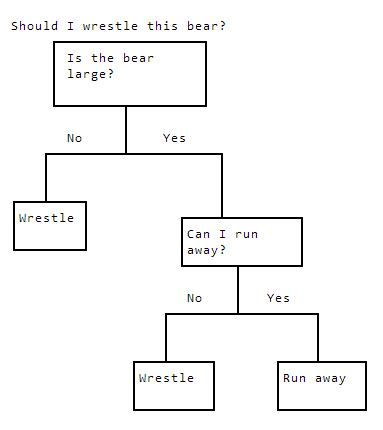
In the diagram above, we're deciding if we should wrestle a bear that's in front of us. We're using various criteria, like the size of the bear, and if escape is possible, to make our final decision. Let's say we had a dataset of people who survived bear encounters, and the actions they took:

 

Bear name    Size    Escape possible?    Action

Yogi         Small   No                  Wrestle

Winnie       Small   Yes                 Wrestle

Baloo        Large   Yes                 Run away

Gentle Ben   Large   No                  Wrestle

If we wanted to optimize our chances of surviving a bear encounter, we could construct a decision tree to tell us what action to take.

As our dataset gets larger though, this gets less and less practical. What if we had 10000 rows and 10 variables? Would you want to look through all the possibilities to construct a tree?

This is where the decision tree machine learning algorithm can help. It enables us to automatically construct a decision tree to tell us what outcomes we should predict in certain situations.

The decision tree algorithm is a supervised learning algorithm -- we first construct the tree with historical data, and then use it to predict an outcome. One of the major advantages of decision trees is that they can pick up nonlinear interactions between variables in the data that linear regression can't. In our bear wrestling example, a decision tree can pick up on the fact that you should only run away from large bears when escape is impossible, whereas a linear regression would have had to weight both factors in the absence of the other.

Trees can be used for classification or regression problems. In this lesson, we'll walk through the building blocks of making a decision tree automatically.

2: Our Dataset

We'll be looking at individual income in the United States. The data is from the 1994 Census, and contains information on an individual's marital status, age, type of work, and more. The target column, or what we want to predict, is if they make less than or equal to 50k a year, or more than 50k a year.

You can download the data from here.

Instructions

This step is a demo. Play around with code or advance to the next step.

import pandas

# Set index_col to False to avoid pandas thinking that the first column is row indexes (it's age).
income = pandas.read_csv("income.csv", index_col=False)
print(income.head(5))

3: Converting Categorical Variables

As we can see in our data, we have categorical variables such as workclass. The values are strings, but one string label can be shared between multiple individuals. The types of work we can do are State-gov, Self-emp-not-inc, Private, and so on. Each one of these strings is a label for a category. Another example of a column of categories is sex, where the options are Male and Female.

Before we get started with decision trees, we need to convert the categorical variables in our dataset to numeric variables. This involves assigning a number to each category label, and converting all the labels in a column to numbers.

When we construct a decision tree, we'll need to be able to deal with numbers. We can accomplish this by converting back and forth to numbers when we construct our decision tree. This is fairly cumbersome, however, so doing this conversion upfront will save us time.

Another strategy is to convert the columns to a categorical type. With this, Pandas will display the labels as strings, but internally store them as numbers so computations can be done with them. This is not always compatible with other libraries, such as Scikit-learn, so it's easier to just do the conversion to numeric upfront.

We can use the Categorical.from_array method from Pandas to perform the conversion to numbers.

Instructions

• Convert the rest of the categorical columns in income (education,marital_status, occupation,relationship, race, sex,native_country, andhigh_income) to numeric columns.

import pandas

# Set index_col to False to avoid pandas thinking that the first column is row indexes (it's age).
income = pandas.read_csv("income.csv", index_col=False)
print(income.head(5))

 

3: Converting Categorical Variables

As we can see in our data, we have categorical variables such as workclass. The values are strings, but one string label can be shared between multiple individuals. The types of work we can do are State-gov, Self-emp-not-inc, Private, and so on. Each one of these strings is a label for a category. Another example of a column of categories is sex, where the options are Male and Female.

Before we get started with decision trees, we need to convert the categorical variables in our dataset to numeric variables. This involves assigning a number to each category label, and converting all the labels in a column to numbers.

When we construct a decision tree, we'll need to be able to deal with numbers. We can accomplish this by converting back and forth to numbers when we construct our decision tree. This is fairly cumbersome, however, so doing this conversion upfront will save us time.

Another strategy is to convert the columns to a categorical type. With this, Pandas will display the labels as strings, but internally store them as numbers so computations can be done with them. This is not always compatible with other libraries, such as Scikit-learn, so it's easier to just do the conversion to numeric upfront.

We can use the Categorical.from_array method from Pandas to perform the conversion to numbers.

Instructions

• Convert the rest of the categorical columns in income (education,marital_status, occupation,relationship, race, sex,native_country, andhigh_income) to numeric columns.

# Convert a single column from text categories into numbers.
col = pandas.Categorical.from_array(income["workclass"])
income["workclass"] = col.codes
print(income["workclass"].head(5))
for name in ["education", "marital_status", "occupation", "relationship", "race", "sex", "native_country", "high_income"]:
    col = pandas.Categorical.from_array(income[name])
    income[name] = col.codes

 

4: Split Points

A decision tree is constructed through a series of nodes and branches. A node is where we split the data based on a variable, and a branch is one side of the split. Here's an example:

Whatincomedopeoplemake?DotheyworkinthePrivatesector?NoYes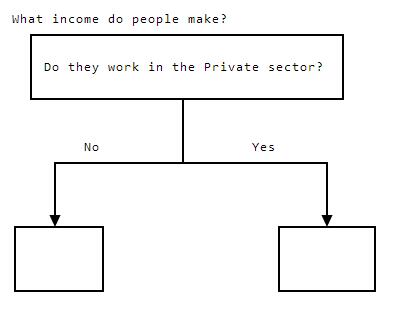

In the above diagram, the node is splitting the data based on if the individual works in the private sector. There are two branches, No, andYes. The workclass column indicates the sector people work in. The value Private in that column has been mapped to the numeric code 4 (we can check this by comparing the values in the workclass column that used to be labelled Private with the current values to see where they line up). So the No branch corresponds to workclass != 4, and the Yes branch corresponds to workclass == 4.

This is exactly how a decision tree works -- we keep splitting the data based on variables. As we do this, the tree gets deeper and deeper. The tree we made above is two levels deep, because it has one split, and two "levels" of nodes.

The tree below is 3 levels deep.

Whatincomedopeoplemake?DotheyworkinthePrivatesector?NoYesNativetotheUS?NoYes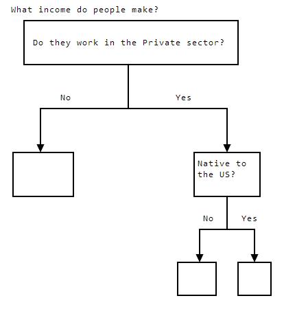

In the tree above, we added another split point, which came "below", or after, our first split point. This made the tree deeper, and the tree is now 3 levels deep.

5: Performing A Split

Now, think of rows of data flowing through a decision tree. In the diagram above, we can split the dataset into two portions based on whether the individual works in the private sector or not.

Instructions

Split income into two parts based on the value of the workclass column.

• private_incomes should contain all rows whereworkclass is 4.
• public_incomes should contain all rows where workclass is not4.

# Enter your code here.
private_incomes = income[income["workclass"] == 4]
public_incomes = income[income["workclass"] != 4]

print(private_incomes.shape)
print(public_incomes.shape)

6: Thinking About The Data

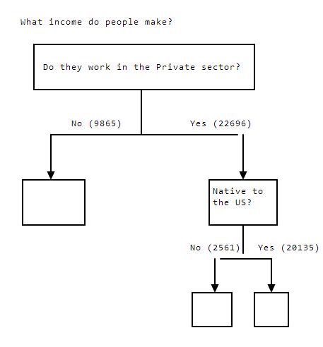
When we performed the split, 9865 rows went to the left, where workclass does not equal 4, and 22696 rows went to the right, where workclass equals 4.

It's useful to think of a decision tree as a flow of rows of data. When we make a split, some rows will go to the right, and some rows will go to the left. As we build the tree deeper and deeper, each node will "receive" less and less rows.

Here's a look at the splits, and the number of rows that will exist at each node:

Whatincomedopeoplemake?DotheyworkinthePrivatesector?No(9865)Yes(22696)NativetotheUS?No(2561)Yes(20135)

7: Rationale Behind Splitting

The nodes at the bottom of the tree, when we decide to stop splitting, are called terminal nodes, or leaves. When we do our splits, we aren't doing them randomly -- we have an objective. Our goal is to ensure that we can make a prediction on future data. In order to do this, all rows in each leaf must have only one value for our target column.

We're trying to predict the high_income column.
If high_income is 1, it means that the person has an income higher than 50k a year.
If high_income is 0, it means that they have an income less than or equal to 50k a year.

After constructing a tree using the income data, we'll want to make predictions. In order to do this, we'll take a new row, and feed it through our decision tree. We'll check to see if the person works in the private sector. If they do, we'll check to see if they are native to the US, and so on.

We'll eventually reach a leaf. The leaf will tell us what value we should predict for high_income.

In order to be able to make this prediction, all leaves need to have rows with only a single value for high_income. So leaves can't have both0 and 1 values in the high_income column. Each leaf can only have rows with the same values for our target. If this doesn't happen, we won't be able to make effective predictions.

So, we keep splitting nodes until we get to a point where all the rows in a node have the same value for high_income.

8: Entropy

Now that we have a high-level view of how decision trees work, let's get into the details and figure out how to perform the splits.

In order to do this, we'll use a measure to figure out which variable to split a node on. Post-split, we'll have two datasets, each containing the rows from one side of the split.

Since we're trying to get to leaves consisting of only 1s or only 0s for high_income, each split will need to get us closer to that goal.

When we split, we'll try to separate as many 0s from 1s in the high_income column as we can. In order to do this, we need a metric for how "together" the different values in the high_income column are.

A commonly used metric is called entropy. Entropy refers to disorder. The more "mixed together" 1s and 0s are, the higher the entropy. A dataset consisting of only 1s in the high_income column would have low entropy.

Entropy, which is not to be confused with entropy from physics, comes from information theory. Information theory is based on probability and statistics, and deals with the transmission, processing, utilization, and extraction of information. A key concept in this is the notion of a bit of information. One bit of information is one unit of information. It can be represented as a binary number -- a bit of information either has the value 1, or 0. If there's an equal probability of tomorrow being sunny (1) and tomorrow being not sunny (0), if I tell you that it will be be sunny, I've given you one bit of information.

Entropy can also be thought of in terms of information. If we flip a coin where both sides are heads, we know upfront that the result will be heads. Thus, we gain no new information by flipping the coin, so entropy is 0. On the other hand, if the coin has a heads side and a tails side, there's a 50% probability of landing on either. Thus, flipping the coin gives us one bit of information -- which side the coin landed on. There's much more complexity, especially when you get to cases with more than two possible outcomes, or differential probabilities. However, a deep understanding of entropy isn't necessary for constructing decision trees. You can read more here if you want.

The formula for entropy is below:

−∑ci=1P(xi)logbP(xi)−∑i=1cP(xi)logb⁡P(xi)

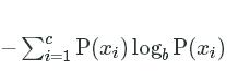
We iterate through each unique value in a single column (in this case, high_income), and assign it to ii. We then compute the probability of that value occurring in the data (P(xi)P(xi)). We then do some multiplication, and all of the values together. bb is the base of the logarithm.2 is a commonly used value for this, but it can also be set to 10 or another value.

Let's say we have this data:

 

age    high_income

25     1

50     1

30     0

50     0

80     1

We could compute the entropy:

−∑i=1cP(xi)logbP(xi)−((2/5∗log22/5)+(3/5∗log23/5))−(−0.5287712379549449+−0.44217935649972373).97−∑i=1cP(xi)logb⁡P(xi)−((2/5∗log2⁡2/5)+(3/5∗log2⁡3/5))−(−0.5287712379549449+−0.44217935649972373).97

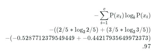
We get less than one "bit" of information -- we only get .97. This is because there are slightly more 1s in the sample data than 0s. This means that if we were predicting a new value, we could guess that the answer is 1, and be right more often than we're wrong (there's a .6 probability of the answer being 1). Because of this prior knowledge, we gain less than a full "bit" of information when we observe a new value.

Instructions

• Compute the entropy of thehigh_income column in theincome dataframe and assign the result to income_entropy.

import math
# We'll do the same calculation we did above, but in Python.
# Passing 2 as the second parameter to math.log will take a base 2 log.
entropy = -(2/5 * math.log(2/5, 2) + 3/5 * math.log(3/5, 2))
print(entropy)
prob_0 = income[income["high_income"] == 0].shape[0] / income.shape[0]
prob_1 = income[income["high_income"] == 1].shape[0] / income.shape[0]
income_entropy = -(prob_0 * math.log(prob_0, 2) + prob_1 * math.log(prob_1, 2))

9: Information Gain
We'll need a way to go from computing entropy to figuring out which variable to split based on. We can do this using information gain. Information gain tells us which split will reduce entropy the most.

Here's the formula for information gain:

IG(T,A)=Entropy(T)−∑v∈A|Tv||T|⋅Entropy(Tv)IG(T,A)=Entropy(T)−∑v∈A|Tv||T|⋅Entropy(Tv)

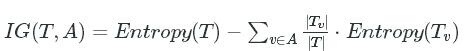
This may look complicated, but we'll break it down. We're computing information gain (IGIG) for a given target variable (TT), and a given variable that we want to split based on (AA). To compute this, we first calculate the entropy for TT. Then, for each unique value vv in the variable AA, we compute the number of rows in which AA takes on the value vv, and divide it by the total number of rows. We then multiply this by the entropy of the rows where AA is vv. We add together all of these subset entropies, and subtract from the overall entropy to get information gain.

For an even simpler explanation, we're finding the entropy of each set post-split, weighting it by the number of items in each split, then subtracting from the current entropy. If it's positive, we've lowered entropy with our split. The higher it is, the more we've lowered entropy.

One strategy to construct trees to is to create as many branches at each node as there are unique values for the variable being split on. So if the variable has 3 or 4 values, that would result in 3 or 4 branches. Usually, this is more complexity than it's worth, and doesn't improve prediction accuracy, but it's worth knowing about.

To simplify the calculation of information gain, and to make splits simpler, we won't do it for each unique value. Instead, for the variable we're splitting on, we'll find the median. Any rows where the value of the variable is below the median will split left, and the rest of the rows will split right. To compute information gain, we'll only have to compute entropies for two subsets.

Here's an example, using the same dataset we did earlier:

age    high_income
25     1
50     1
30     0
50     0
80     1
Let's say we wanted to split this dataset based on age. First, we calculate the median age, which is 50. Then, we assign any row with a value less than or equal to the median age 0, and the other rows 1.

age    high_income    split_age
25     1              0
50     1              0
30     0              0
50     0              0
80     1              1
Now we compute entropy:

IG(T,A)=Entropy(T)−∑v∈A|Tv||T|⋅Entropy(Tv).97−(((4/5)∗−(1/2∗log21/2+1/2∗log21/2))+−(1/5∗(0∗log20+1∗log21))).97−((4/5)∗−(−.5+−.5))+(1/5∗−(0+1∗0)).97−(4/5).169IG(T,A)=Entropy(T)−∑v∈A|Tv||T|⋅Entropy(Tv).97−(((4/5)∗−(1/2∗log21/2+1/2∗log21/2))+−(1/5∗(0∗log20+1∗log21))).97−((4/5)∗−(−.5+−.5))+(1/5∗−(0+1∗0)).97−(4/5).169

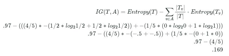
We end up with .17, which means that we gain .17 bits of information by splitting our dataset on the age variable.

Instructions
Compute the information gain for splitting on the age column of income.
First, compute the median of age.
Then, assign anything less than or equal to the median to the left split, and anything greater than the median to the right split.
Compute the information gain and assign to age_information_gain.

 

import numpy

def calc_entropy(column):
    """
    Calculate entropy given a pandas Series, list, or numpy array.
    """
    # Compute the counts of each unique value in the column.
    counts = numpy.bincount(column)
    # Divide by the total column length to get a probability.
    probabilities = counts / len(column)
    
    # Initialize the entropy to 0.
    entropy = 0
    # Loop through the probabilities, and add each one to the total entropy.
    for prob in probabilities:
        if prob > 0:
            entropy += prob * math.log(prob, 2)
    
    return -entropy

# Verify our function matches our answer from earlier.
entropy = calc_entropy([1,1,0,0,1])
print(entropy)

information_gain = entropy - ((.8 * calc_entropy([1,1,0,0])) + (.2 * calc_entropy([1])))
print(information_gain)
income_entropy = calc_entropy(income["high_income"])

median_age = income["age"].median()

left_split = income[income["age"] <= median_age]
right_split = income[income["age"] > median_age]

age_information_gain = income_entropy - ((left_split.shape[0] / income.shape[0]) * calc_entropy(left_split["high_income"]) + ((right_split.shape[0] / income.shape[0]) * calc_entropy(right_split["high_income"])))

 

10: Finding The Best Split

Now that we know how to compute information gain, we can compute the best variable to split a node on. When we start our tree, we want to make an initial split. We'll find the variable to split on by finding which split would have the highest information gain.

Instructions

Make a list called information_gains.

• It should contain, in order, the information gain from splitting on these columns: age, workclass, education_num, marital_status, occupation, relationship, race, sex, hours_per_week, native_country.

Find the highest value in theinformation_gains list and assign this column name to highest_gain.

def calc_information_gain(data, split_name, target_name):
    """
    Calculate information gain given a dataset, column to split on, and target.
    """
    # Calculate original entropy.
    original_entropy = calc_entropy(data[target_name])
    
    # Find the median of the column we're splitting.
    column = data[split_name]
    median = column.median()
    
    # Make two subsets of the data based on the median.
    left_split = data[column <= median]
    right_split = data[column > median]
    
    # Loop through the splits, and calculate the subset entropy.
    to_subtract = 0
    for subset in [left_split, right_split]:
        prob = (subset.shape[0] / data.shape[0]) 
        to_subtract += prob * calc_entropy(subset[target_name])
    
    # Return information gain.
    return original_entropy - to_subtract

# Verify that our answer is the same as in the last screen.
print(calc_information_gain(income, "age", "high_income"))

columns = ["age", "workclass", "education_num", "marital_status", "occupation", "relationship", "race", "sex", "hours_per_week", "native_country"]
information_gains = []
# Loop through and compute information gains.
for col in columns:
    information_gain = calc_information_gain(income, col, "high_income")
    information_gains.append(information_gain)

# Find the name of the column with the highest gain.
highest_gain_index = information_gains.index(max(information_gains))
highest_gain = columns[highest_gain_index]

11: Build The Whole Tree

We now know how to make a single split. In order to construct a tree, we'll need to construct these splits all the way down the tree, until the leaves only have a single class.

Here's an example:

 

age    high_income

25     1

50     1

30     0

50     0

80     1

Incomevs.AgeOver50?No(4)Yes(1)Over40?Leaf(1)No(2)Yes(2)Over27?Leaf(.5)NYesLeaf(1)Leaf(0)

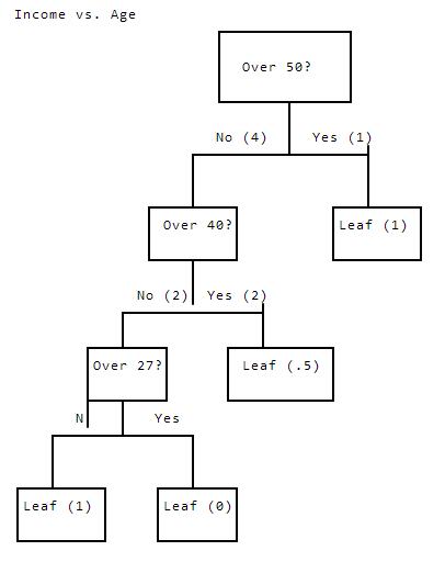
As we see above, we split the data all the way down. This example is different, because we only have a single variable to split with. This results in one leaf where both rows have age 50, so we can't split, but one has high_income of 1, and the other has high_income of0. In this case, we would usually be able to split on another variable, but if that's not possible, we would predict .5 for any rows we were predicting on that ended up at this leaf.

In order to construct a tree like this, we'll need to be able to split each node multiple times.

12: Conclusion

So far, we've been following the ID3 algorithm to construct decision trees. There are other algorithms, including CART that use other measures for the split criterion. We'll learn more about these other algorithms in future missions.

In the next mission, we'll figure out how to recursively construct an entire tree, using the ID3 algorithm.

转载于:https://my.oschina.net/Bettyty/blog/752934