Unsupervised Learning and Text Mining of Emotion Terms Using R

Unsupervised learning refers to data science approaches that involve learning without a prior knowledge about the classification of sample data. In Wikipedia, unsupervised learning has been described as “the task of inferring a function to describe hidden structure from ‘unlabeled’ data (a classification of categorization is not included in the observations)”. The overarching objectives of this post were to evaluate and understand the co-occurrence and/or co-expression of emotion words in individual letters, and if there were any differential expression profiles /patterns of emotions words among the 40 annual shareholder letters? Differential expression of emotion words was being used to refer to quantitative differences in emotion word frequency counts among letters, as well as qualitative differences in certain emotion words occurring uniquely in some letters but not present in others.

The dataset

This is the second part to a companion post I have on “parsing textual data for emotion terms”. As with the first post, the raw text data set for this analysis was using Mr. Warren Buffett’s annual shareholder letters in the past 40-years (1977 – 2016). The R code to retrieve the letters was from here.

## Retrieve the letters  
library(pdftools)      
library(rvest)       
library(XML)
# Getting & Reading in HTML Letters
urls_77_97 <- paste('http://www.berkshirehathaway.com/letters/', seq(1977, 1997), '.html', sep='')
html_urls <- c(urls_77_97,
               'http://www.berkshirehathaway.com/letters/1998htm.html',
               'http://www.berkshirehathaway.com/letters/1999htm.html',
               'http://www.berkshirehathaway.com/2000ar/2000letter.html',
               'http://www.berkshirehathaway.com/2001ar/2001letter.html')

letters_html <- lapply(html_urls, function(x) read_html(x) %>% html_text())
# Getting & Reading in PDF Letters
urls_03_16 <- paste('http://www.berkshirehathaway.com/letters/', seq(2003, 2016), 'ltr.pdf', sep = '')
pdf_urls <- data.frame('year' = seq(2002, 2016),
                       'link' = c('http://www.berkshirehathaway.com/letters/2002pdf.pdf', urls_03_16))
download_pdfs <- function(x) {
  myfile = paste0(x['year'], '.pdf')
  download.file(url = x['link'], destfile = myfile, mode = 'wb')
  return(myfile)
}
pdfs <- apply(pdf_urls, 1, download_pdfs)
letters_pdf <- lapply(pdfs, function(x) pdf_text(x) %>% paste(collapse=" "))
tmp <- lapply(pdfs, function(x) if(file.exists(x)) file.remove(x)) 
# Combine letters in a data frame
letters <- do.call(rbind, Map(data.frame, year=seq(1977, 2016), text=c(letters_html, letters_pdf)))
letters$text <- as.character(letters$text)

Analysis of emotions terms usage

## Load additional required packages
require(tidyverse)
require(tidytext)
require(gplots)
require(SnowballC)
require(sqldf)
theme_set(theme_bw(12))
### pull emotion words and aggregate by year and emotion terms

emotions <- letters %>%
  unnest_tokens(word, text) %>%                           
  anti_join(stop_words, by = "word") %>%                  
  filter(!grepl('[0-9]', word)) %>%
  left_join(get_sentiments("nrc"), by = "word") %>%
  filter(!(sentiment == "negative" | sentiment == "positive")) %>%
  group_by(year, sentiment) %>%
  summarize( freq = n()) %>%
  mutate(percent=round(freq/sum(freq)*100)) %>%
  select(-freq) %>%
  spread(sentiment, percent, fill=0) %>%
  ungroup()
## Normalize data 
sd_scale <- function(x) {
     (x - mean(x))/sd(x)
 }
emotions[,c(2:9)] <- apply(emotions[,c(2:9)], 2, sd_scale)
emotions <- as.data.frame(emotions)
rownames(emotions) <- emotions[,1]
emotions3 <- emotions[,-1]
emotions3 <- as.matrix(emotions3)
## Using a heatmap and clustering to visualize and profile emotion terms expression data

heatmap.2(
     emotions3,
     dendrogram = "both",
     scale      = "none",
     trace      = "none",
     key        = TRUE,
     col    = colorRampPalette(c("green", "yellow", "red"))
 )

Heatmap and clustering: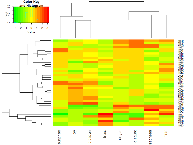

The colors of the heatmap represent high levels of emotion terms expression (red), low levels of emotion terms expression (green) and average or moderate levels of emotion terms expression (yellow).

Co-expression profiles of emotion words usage

Based on the expression profiles combined with the vertical dendrogram, there are about four co-expression profiles of emotion terms: i) emotion terms referring to fear and sadness appeared to be co-expressed together, ii) anger and disgust showed similar expression profiles and hence were co-expressed emotion terms; iii) emotion terms referring to joy, anticipation and surprise appeared to be similarly expressed, and iv) emotion terms referring to trust did show the least co-expression pattern.

Emotion expression profiling of annual shareholder letters

Looking at the horizontal dendrogram and heatmap above, approximately six groups of emotions expressions profiles can be recognized among the 40 annual shareholder letters.
Group-1 letters showed over-expression of emotion terms referring to anger, disgust, sadness or fear. Letters of this group included 1982, 1987, 1989 & 2003 (first 4 rows of the heatmap).
Group-2 and group-3 letters showed over-expression of emotion terms referring to surprise, disgust, anger and sadness. Letters of this group included 1985, 1994, 1996, 1998, 2010, 2014, 2016, 1990 – 1993, 2002, 2004, 2005 & 2015 (rows 5 – 19 of the heatmap).
Group-4 letters showed over-expression of emotion terms referring to surprise, joy and anticipation. Letters of this group included 1995, 1997 – 2000, 2006, 2007, 2009 & 2011 – 2013 (rows 20 – 30).
Group-5 letters showed over-expression of emotion terms referring to fear, sadness, anger and disgust. Letters of this group included 1984, 1986, 2001 & 2008 (rows 31 – 34).
Group-6 letters showed over-expression of emotion terms referring to trust. Letters of this group included those of the early letters (1977 – 1981 & 1983) (rows 35 – 40).

Numbers of emotion terms expressed uniquely or in common among the heatmap groups

The next steps of the analysis attempted to determine the numbers of emotion words that were uniquely expressed in any of the heatmap groups. Also wanted to see if some emotion words were expressed in all of the heatmap groups, if any? For these analyses, I chose to include a word stemming procedure. Wikipedia described word stemming as “the process of reducing inflected (or sometimes derived) words to their word stem, base or root form- generally a written word form”. In practice, the stemming step removes word endings such as “es”, “ed” and “’s”, so that the various word forms would be taken as same when considering uniqueness and/or counting word frequency (see the example below for before and after applying word stemmer function in R).

Examples of word stemmer output

There are several word stemmers in R. One such function, the wordStem, in the SnowballC package extracts the stems of each of the given words in a vector (See example below).

Before <- c("produce",  "produces", "produced", "producing", "product", "products", "production")
wstem <- as.data.frame(wordStem(Before))
names(wstem) <- "After"
pander::pandoc.table(cbind(Before, wstem))
Here is the example output for stemming
## ------------------
##   Before    After 
## ---------- -------
##  produce   produc 
## 
##  produces  produc 
## 
##  produced  produc 
## 
## producing  produc 
## 
##  product   product
## 
##  products  product
## 
## production product
## ------------------

Analysis of unique and commonly expressed emotion words

## pull emotions words for selected heatmap groups and apply stemming
set.seed(456)
emotions_final <- letters  %>%
   unnest_tokens(word, text) %>% 
filter(!grepl('[0-9]', word)) %>%                          
   left_join(get_sentiments("nrc"), by = "word") %>%
filter(!(sentiment == "negative" | sentiment == "positive" | sentiment == "NA")) %>%
subset(year==1987 | year==1989 |  year==2001 |  year==2008 | year==2012 | year==2013) %>%
mutate(word = wordStem(word)) %>%
ungroup()
group1 <- emotions_final %>% 
     subset(year==1987| year==1989 ) %>%
     select(-year, -sentiment) %>%
     unique()
set.seed(456)
group4 <- emotions_final %>% 
     subset(year==2012 | year==2013) %>%
     select(-year, -sentiment) %>%
     unique()
set.seed(456)
group5 <- emotions_final %>%
     subset(year==2001 | year==2008 ) %>%
     select(-year, -sentiment) %>%
     unique()

Unique and common emotion words among two groups

Let’s draw a two-way Venn diagram to find out which emotions terms were unique or commonly expressed between heatmap group-1 & group-4.

# common and unique words between two groups
emo_venn2 <- venn(list(group1$word, group4$word))

Two-way Venn diagram:

A total of 293 emotion terms were expressed in common between group-1 (A) and group-4 (B). There were also 298 and 162 unique emotion words usage in heatmap groups-1 & 4, respectively.

Unique and common emotion words among three groups

Let’s draw a three way Venn diagram to find out which emotions terms were uniquely or commonly expressed among group-1, group-4 & group-5.

# common and unique words among three groups
emo_venn3 <- venn(list(group1$word, group4$word, group5$word))

Three way Venn diagram:

A total of 225 emotion terms were expressed in common among the three heatmap groups. On the other hand, there were 193, 108 and 159 unique emotion words usage in heatmap group-1 (A), group-4 (B) and group-5 (C), respectively. The Venn diagram included various combinations of unique and common emotion word expressions. Of particular interest were the 105 emotion words that were expressed in common between heatmap group-1 and group-5. Recall that group-1 & group-5 were highlighted for their high expression of emotions referring to disgust, anger, sadness and fear.

I also wanted to see a list of those emotion words that were expressed uniquely and/or in common among several groups. For instance the R code below requested for a list of the 109 unique emotion words that were expressed solely in group-5 letters of the 2001 & 2008.

## The code below pulled a list of all common/unique emotion words expressed
## in all possible combinations of the the three heatmap groups
venn_list <- (attr(emo_venn3, "intersection"))
## and then print only the list of unique emotion words expressed in group-5.
print(venn_list$'C')
##   [1] "manual"          "familiar"        "sentenc"        
##   [4] "variabl"         "safeguard"       "abu"            
##   [7] "egregi"          "gorgeou"         "hesit"          
##  [10] "strive"          "loyalti"         "loom"           
##  [13] "approv"          "like"            "winner"         
##  [16] "entertain"       "tender"          "withdraw"       
##  [19] "harm"            "strike"          "straightforward"
##  [22] "victim"          "iron"            "bounti"         
##  [25] "chaotic"         "bloat"           "proviso"        
##  [28] "frank"           "honor"           "child"          
##  [31] "lemon"           "prospect"        "relev"          
##  [34] "threaten"        "terror"          "quak"           
##  [37] "scarciti"        "question"        "manipul"        
##  [40] "deton"           "terrorist"       "attack"         
##  [43] "ill"             "nation"          "hydra"          
##  [46] "disast"          "sadli"           "prolong"        
##  [49] "concern"         "urgenc"          "presid"         

The output from the above code included a list of 159 words, but the list above contained only the first 51 for space considerations. Besides, you may have noticed that some of the emotions words were truncated and did not look proper words due to stemming.

Dispersion Plot

Dispersion plot is a graphical display that can be used to represent the approximate locations and densities of emotion terms across the length of the text document. Shown below are three dispersion plots of unique emotion words of heatmap group-1 (1987, 1989), group-5 (2001, 2008) and group-4 (2012 and 2013) shareholder letters. For the dispersion plots, all words in the listed years were sequentially ordered by year of the letters and the presence and approximate locations of the unique words were identified/displayed by a stripe. Each stripe represented an instance of a unique word in the shareholder letters.

Confirmation of emotion words expressed uniquely in heatmap group-1

## Confirmation of unique emotion words in heatmap group-1
group1_U <- as.data.frame(venn_list$'A')
names(group1_U) <- "terms"
uniq1 <- sqldf( "select t1.*, g1.terms
from emotions_final t1
left join
group1_U g1
on t1.word = g1.terms "
)
uniq1a <- !is.na(uniq1$terms)
uniqs1 <- rep(NA, length(emotions_final))
uniqs1[uniq1a] <- 1
plot(uniqs1, main="Dispersion plot of emotions words \n unique to heatmap group 1 ", xlab="Length (Word count)", ylab=" ", col="red", type='h', ylim=c(0,1), yaxt='n')

Heatmap plot: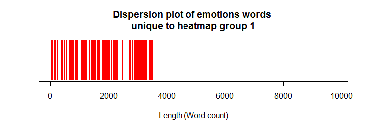

Heatmap group-1 letters included those in 1987/1989. As expected, the dispersion plot above confirmed that the unique emotion words in group-1 were confined at the start of the dispersion plot.

Confirmation of emotion words expressed uniquely in heatmap group-5

## confirmation of unique emotion words in heatmap group-5  
group5_U <- as.data.frame(venn_list$'C')
names(group5_U) <- "terms"
uniq5 <- sqldf( "select t1.*, g5.terms
from emotions_final t1
left join
group5_U g5
on t1.word = g5.terms "
)
uniq5a <- !is.na(uniq5$terms)
uniqs5 <- rep(NA, length(emotions_final))
uniqs5[uniq5a] <- 1
 
plot(uniqs5, main="Dispersion plot of emotions words \n unique to heatmap group 5 ", xlab="Length (Word count)", ylab=" ", col="red", type='h', ylim=c(0,1), yaxt='n')

Dispersion plot of emotions words: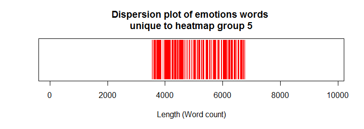

Heatmap group-5 letters included those in 2001 & 2008. As expected, the dispersion plot above confirmed that the unique emotion words in group-5 were confined at the middle parts of the dispersion plot.

Confirmation of emotion words expressed uniquely in heatmap group-4

## confirmation of unique emotion words in heatmap group-4 
group4_U <- as.data.frame(venn_list$'B')
names(group4_U) <- "terms"
uniq4 <- sqldf( "select t1.*, g4.terms
from emotions_final t1
left join
group4_U g4
on t1.word = g4.terms "
)
uniq4a <- !is.na(uniq4$terms)
uniqs4 <- rep(NA, length(emotions_final))
uniqs4[uniq4a] <- 1

plot(uniqs4, main="Dispersion plot of emotions words \n unique to heatmap group 4 ", xlab="Length (Word count)", ylab=" ", col="red", type='h', ylim=c(0,1), yaxt='n')

Dispersion plot of emotions words: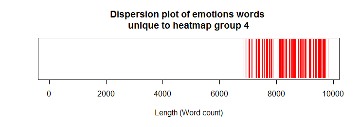

Heatmap group4 letters included those in 2012 & 2013. As expected, the dispersion plot above confirmed that the unique emotion words in group-4 were confined towards the end of the dispersion plot.

Annual Returns on Investment in S&P500 (1977 – 2016)

Finally a graph of the annual returns on investment in S&P 500 during the same 40 years of the annual shareholder letters is being displayed below for perspective. The S&P 500 data was downloaded from here using an R code from here.

## You need to first download the raw data before running the code to recreate the graph below. 
ggplot(sp500[50:89,], aes(x=year, y=return, colour=return>0)) +
geom_segment(aes(x=year, xend=year, y=0, yend=return),
size=1.1, alpha=0.8) +
geom_point(size=1.0) +
xlab("Investment Year") +
     ylab("S&P500 Annual Returns") +
     labs(title="Annual Returns on Investment in S&P500", subtitle= "source: http://pages.stern.nyu.edu/~adamodar/New_Home_Page/datafile/histretSP.html") + 
     theme(legend.position="none") +
     coord_flip()

Annual Returns on Investment in S&P500:

Concluding Remarks

R offers several packages and functions for the evaluation and analyses of differential expression and co-expression profiling of emotion words in textual data, as well as visualization and presentation of analyses results. Some of those functions, techniques and tools have been attempted in two companion posts. Hopefully, you found the examples helpful.

转自：https://datascienceplus.com/unsupervised-learning-and-text-mining-of-emotion-terms-using-r/

转载于:https://www.cnblogs.com/payton/p/6877171.html