python 小波_Matlab 小波功率谱&Python小波分析

%相关调用函数百度一下随处可见clc;clear;close alldata=load('tangyrtem1.txt');sst=data(:,2);variance = std(sst)^2;sst = (sst - mean(sst))/sqrt(variance) ;n = length(sst);dt = 1.0; %每个数据之间的时间步长。time = data(:,1);  % construct time array(构造时间数组)xlim = data(1,1)+[1,n-1];  % plotting range(绘图范围)pad = 1;      % pad the time series with zeroes (recommended)(用0填充时间序列(推荐))dj = 0.05;    % this will do 4 sub-octaves per octave; the spacing between discrete scales. Default is 0.25. a smaller # will give better scale resolution, but be slower to plot.(每个八度有四个亚八度;离散尺度之间的距离。默认是0.25。较小的#将提供更好的比例分辨率，但绘图较慢。)s0 = 2*dt;    % this says start at a scale of 6 months(这表示从6个月开始)j1 = 4/dj;    %%  Default is j1 = (LOG2(n DT/S0))/dj.  this says do 7 powers-of-two with dj sub-octaves each   zl：改变纵轴数值 64 128 256...(也就是说1是4，2是8，3是16，4是32，5是64，6是128)lag1 = 0.72;  % lag-1 autocorrelation for red noise backgroundmother = 'morlet';% Wavelet transform(小波变换):[wave,period,scale,coi] = wavelet(sst,dt,pad,dj,s0,j1,mother);power = (abs(wave)).^2 ;        % compute wavelet power spectrum(计算小波功率谱)% Significance levels: (variance=1 for the normalized SST)(显著性水平:(标准化海表温度方差=1))[signif,fft_theor] = wave_signif(1.0,dt,scale,0,lag1,0.90,-1,mother);sig95 = (signif')*(ones(1,n));  % expand signif --> (J+1)x(N) arraysig95 = power ./ sig95;         % where ratio > 1, power is significant% Global wavelet spectrum & significance levels(全局小波频谱及显著性水平):global_ws = variance*(sum(power')/n);   % time-average over all timesdof = n - scale;  % the -scale corrects for padding at edges(-scale修正了边的填充)global_signif = wave_signif(variance,dt,scale,1,lag1,0.90,dof,mother);% Scale-average between El Nino periods of 2--8 yearsavg = find((scale >=10 ) & (scale < 12));                          %zlCdelta = 0.776;   % this is for the MORLET waveletscale_avg = (scale')*(ones(1,n));  % expand scale --> (J+1)x(N) arrayscale_avg = power ./ scale_avg;   % [Eqn(24)]scale_avg = variance*dj*dt/Cdelta*sum(scale_avg(avg,:));   % [Eqn(24)]scaleavg_signif = wave_signif(variance,dt,scale,2,lag1,-1,[10,12],mother);%zl：检验whos%------------------------------------------------------ Plotting%--- Plot time seriessubplot('position',[0.08 0.72 0.65 0.2])          %0.1，0.75：起点；0.65：宽；0.2：高plot(time,sst)set(gca,'XLim',xlim(:))xlabel('Time (year)')ylabel('DegC')title('a) Tang Temperature Original Data')hold onp5 = polyfit(time,sst,1);         % 5 阶多项式拟合 y5 = polyval(p5,time);plot(time,y5,'-r');hold off%--- Contour plot wavelet power spectrumsubplot('position',[0.08 0.1 0.65 0.5])         % subplot('position',[0.15 0.10 0.5 0.6]) levels = [0.0625,0.125,0.25,0.5,1,2,4,8,16] ;Yticks = 2.^(fix(log2(min(period))):fix(log2(max(period))));imagesc(time,log2(period),log2(power));shading interpclim=get(gca,'clim'); %center color limits around log2(1)=0 围绕log2(1)=0的中心颜色限制    clim=[-1 1]*max(clim(2),3);    set(gca,'clim',clim)%contour(time,log2(period),log2(power),log2(levels),'LineWidth',3);  %*** or use 'contourf'% colorbar('position',[0.66 0.08 0.015 0.6],'LineWidth',3,'FontSize',30)%imagesc(time,log2(period),log2(power));  %*** uncomment for 'image' plotxlabel('Time (year)')ylabel('Period (year)')title('b) Wavelet Power Spectrum')set(gca,'XLim',xlim(:))set(gca,'YLim',log2([min(period),max(period)]), ...  'YDir','reverse', ...  'YTick',log2(Yticks(:)), ...  'YTickLabel',Yticks)% 95% significance contour, levels at -99 (fake) and 1 (95% signif)hold oncontour(time,log2(period),sig95,[-99,1],'k','linewidth',1.5);hold on% cone-of-influence, anything "below" is dubiousplot(time,log2(coi),'k')hold off% subplot('position',[left bottem width height])% 表示在当前图形的位置(position)上画图,% 该位置采用归一化的方式,% 即将当前的图形窗口左下角设置为[0,0],% 右上角设置为[1,1],[left bottom width height]中% left表示距离图形窗口左边的距离,% bottom表示距离窗口下边的距离,% width,heigth分别表示绘制坐标轴的大小,% 其中要注意的是left bottom width height这四个值都是0和1之间,刚才也说了,是归一化的坐标.%--- Plot global wavelet spectrumsubplot('position',[0.76 0.1 0.2 0.5])plot(global_ws,log2(period))hold onplot(global_signif,log2(period),'--')hold offxlabel('Power (mm)^2')title('c) Global Wavelet Spectrum')set(gca,'YLim',log2([min(period),max(period)]), ...  'YDir','reverse', ...  'YTick',log2(Yticks(:)), ...  'YTickLabel','')set(gca,'XLim',[0,1.25*max(global_ws)])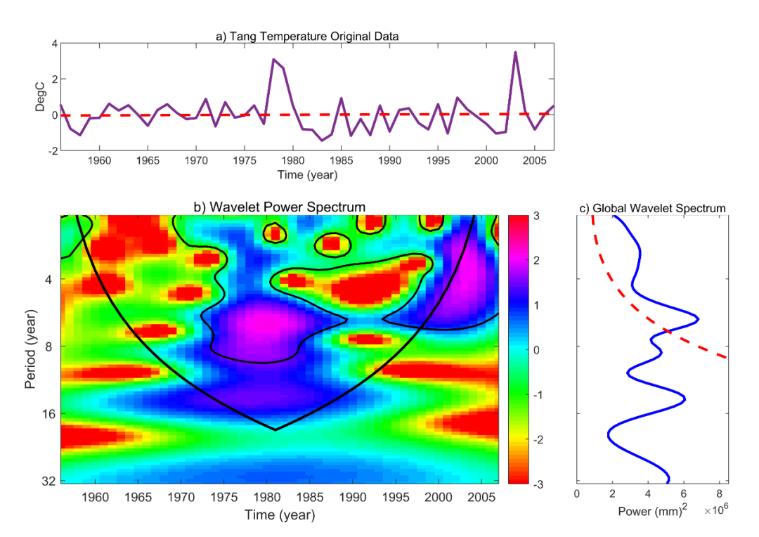

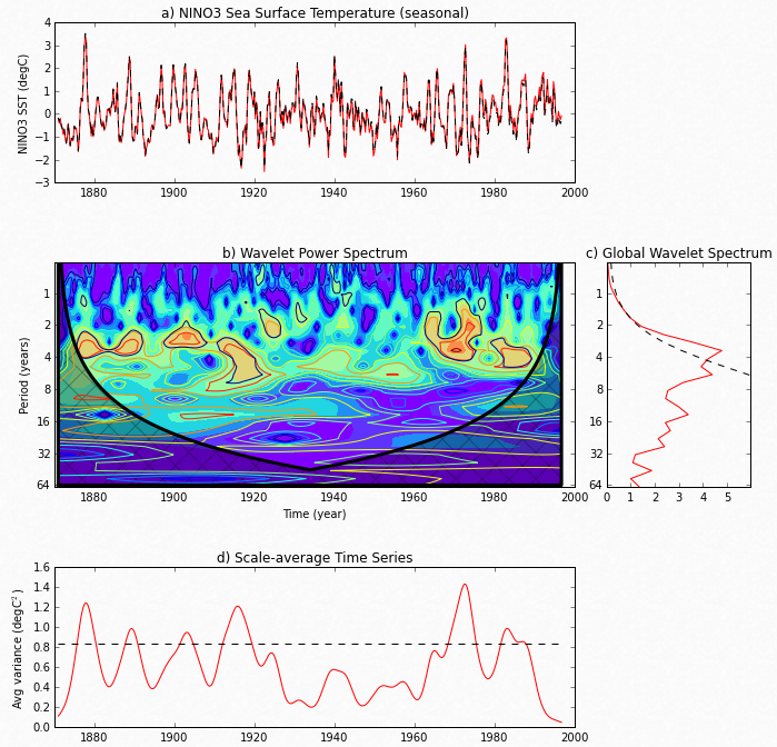
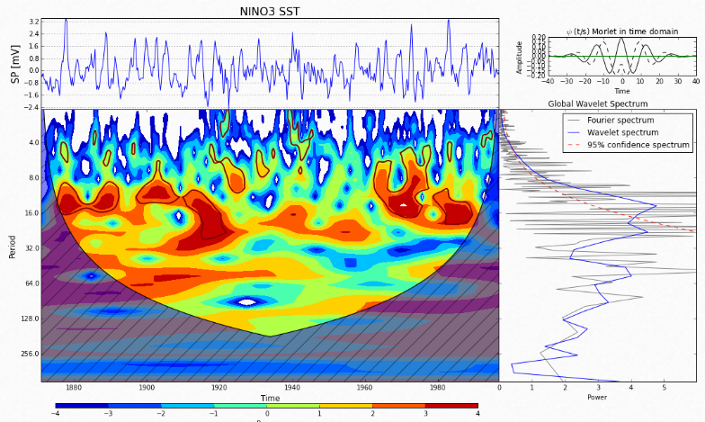
3.2 小波分析Python

http://nicolasfauchereau.github.io/climatecode/posts/wavelet-analysis-in-python/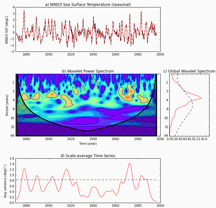

---

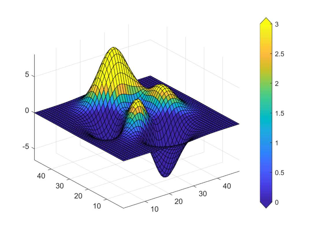
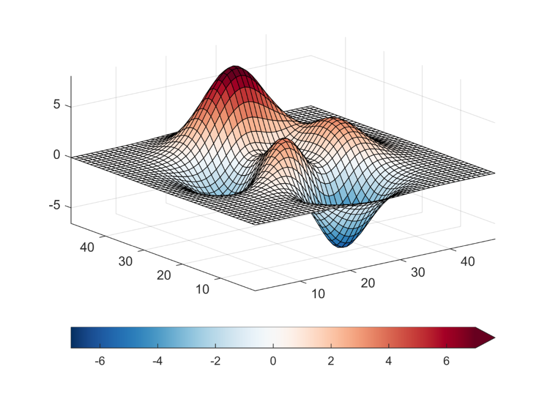
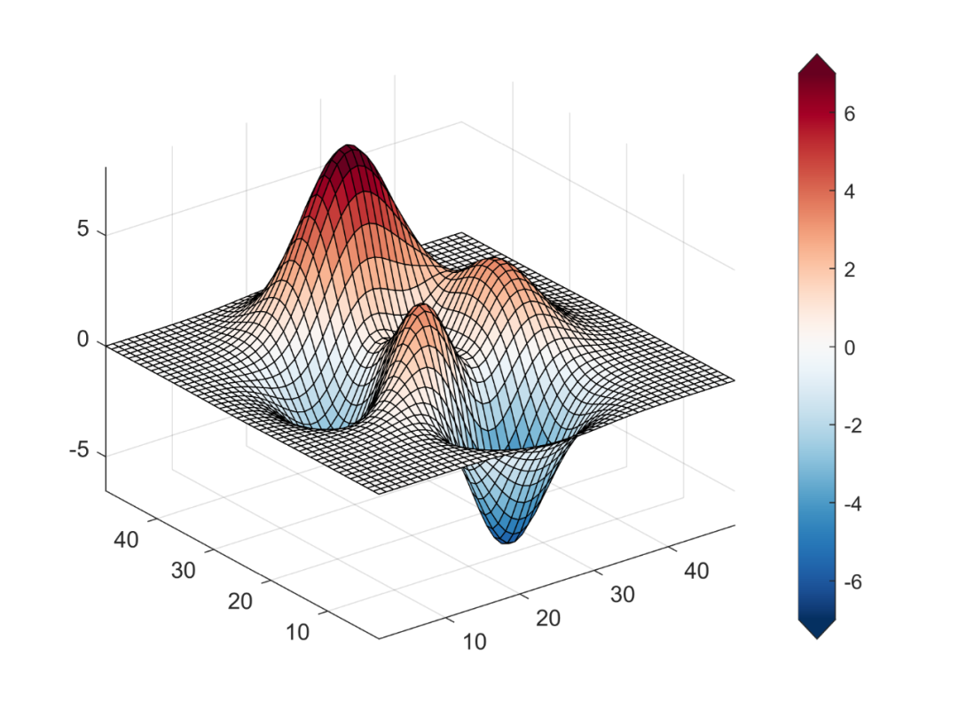
4 Matlab colorbar

clc;clear;close all%%%%%%%%%%%%%%%%%%%%%%%%%%%%%%%%%%%%%%%%%%%%%%%%%%%%%%%%figure(1)surf(peaks);axis tightcolorbar;% colorbar('position',[0.95 0.1 0.04 0.8]);%%%%%%%%%%%%%%%%%%%%%%%%%%%%%%%%%%%%%%%%%%%%%%%%%%%%%%%%figure(2);surf(peaks);axis tightcolorbar;caxis;caxis([0 3]); %%%%%%%%%%%%%%%%%%%%%%%%%%%%%%%%%%%%%%%%%%%%%%%%%%%%%%%%figure(3)surf(peaks);axis tightcolorbar;caxis ;caxis([0 3]) ;cbarrow;%%%%%%%%%%%%%%%%%%%%%%%%%%%%%%%%%%%%%%%%%%%%%%%%%%%%%%%%figure(4)surf(peaks); axis tightcolorbar('southoutside'); colormap(brewermap(256,'*RdBu'));caxis([-7 7]); cbarrow('right');%%%%%%%%%%%%%%%%%%%%%%%%%%%%%%%%%%%%%%%%%%%%%%%%%%%%%%%%figure(5)surf(peaks); axis tightcolorbar('southoutside'); colormap(brewermap(256,'*RdBu'));caxis([-7 7]); cbarrow('left'); %%%%%%%%%%%%%%%%%%%%%%%%%%%%%%%%%%%%%%%%%%%%%%%%%%%%%%%%figure(51)surf(peaks); axis tightcolorbar('southoutside'); colormap(brewermap(256,'*RdBu'));caxis([-7 7]); cbarrow; %%%%%%%%%%%%%%%%%%%%%%%%%%%%%%%%%%%%%%%%%%%%%%%%%%%%%%%%figure(6)surf(peaks); axis tightcolorbar('westoutside'); colormap(brewermap(256,'*RdBu'));caxis([-7 7]); cbarrow; %%%%%%%%%%%%%%%%%%%%%%%%%%%%%%%%%%%%%%%%%%%%%%%%%%%%%%%%figure(7)surf(peaks); axis tightcolorbar('northoutside'); colormap(brewermap(256,'*RdBu'));caxis([-7 7]); cbarrow; %%%%%%%%%%%%%%%%%%%%%%%%%%%%%%%%%%%%%%%%%%%%%%%%%%%%%%%%figure(8)surf(peaks); axis tightcolorbar('eastoutside'); colormap(brewermap(256,'*RdBu'));caxis([-7 7]); cbarrow;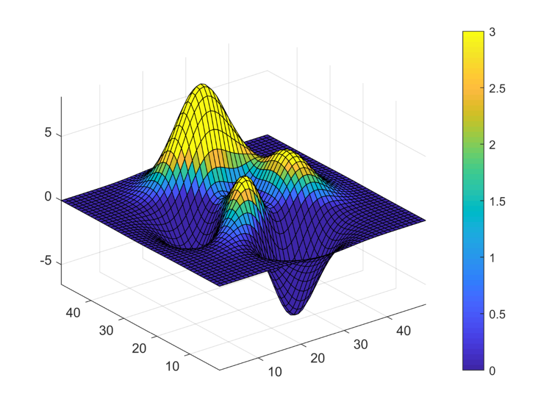

clc;clear;close alltick=-20:5:20;color=[69 117 180;116 173 203;171 217 233;254 224 144;253 174 77;244 109 67;215 48 39;165 0 38]/255;mode='h';colorbarn(tick,color,mode)

function [ax1,c] = colorbarn(tick,color,mode)%---------------------------------%带尖端的colorbar%[ax1,c] = COLORBARN(tick,color,mode)%坐标轴句柄是c,绘图窗句柄是ax1%详情请参考函数 [ax1,c,h]=contf_line(lon,lat,X,tick,color,mode)%---------------------------------[m,~]=size(color);len_tick=length(tick);if len_tick-m ~= 1    returnendfigure;set(gcf,'color','w');if isequal(mode,'h')    c=axes('position',[0.1 0.1 0.8 0.03]);    cdata=zeros(1,m);    for i=1:m        cdata(i)=(tick(i)+tick(i+1))/2;    end    axis([0 m 0 1])    line([0 1],[0 0],'linewidth',2,'color','w','parent',c)    line([m-1 m],[0 0],'linewidth',2,'color','w','parent',c)    colormap(color);    %------------------------    pat_v1=[1 0;1 1;2 1;2 0];pat_f1=reshape(1:(m-2)*4,4,m-2)';    for j=2:m-2        pat_v1=[pat_v1;[j 0;j 1;j+1 1;j+1 0]];    end    pat_col1=[cdata(2:end-1)]';    patch('Faces',pat_f1,'Vertices',pat_v1,'FaceVertexCData',pat_col1,'FaceColor','flat');    %--------------------------------------------------       pat_v2=[0 0.5;1 0;1 1;m-1 1;m-1 0;m 0.5];    pat_f2=[1 2 3;4 5 6];    pat_col2=[cdata(1);cdata(end)];    patch('Faces',pat_f2,'Vertices',pat_v2,'FaceVertexCData',pat_col2,'FaceColor','flat');    %---------------------------------------------------------    set(c,'color','none','xcolor','k','ycolor','none');    box off%     line([1 m-1],[0 0],'color','k')%     line([1 m-1],[1 1],'color','k')%     for i=2:m-2%         line([i i],[0 1],'color','k')%     end    set(c,'xtick',1:m-1,'xticklabel',num2cell(tick(2:end-1)),'ytick',[])    ax1=axes('position',[0.1 0.2 0.8 0.7]);elseif isequal(mode,'v')    c=axes('position',[0.87 0.11 0.02 0.81]);    set(c,'yaxislocation','right');    cdata=zeros(1,m);    for i=1:m        cdata(i)=(tick(i)+tick(i+1))/2;    end    axis([0 1 0 m])    line([1 1],[0 1],'linewidth',2,'color','w','parent',c)    line([1 1],[m-1 m],'linewidth',2,'color','w','parent',c)    colormap(color);    %--------------------------------------------    pat_v1=[0 1;1 1;1 2;0 2];pat_f1=reshape(1:(m-2)*4,4,m-2)';    for j=2:m-2        pat_v1=[pat_v1;[0 j;1 j;1 j+1;0 j+1]];    end    pat_col1=[cdata(2:end-1)]';    patch('Faces',pat_f1,'Vertices',pat_v1,'FaceVertexCData',pat_col1,'FaceColor','flat');    %--------------------------------------------------       pat_v2=[0.5 0;1 1;0 1;1 m-1;0.5 m;0 m-1];    pat_f2=[1 2 3;4 5 6];    pat_col2=[cdata(1);cdata(end)];    patch('Faces',pat_f2,'Vertices',pat_v2,'FaceVertexCData',pat_col2,'FaceColor','flat');    %------------------------------------------------------    set(c,'color','none','xcolor','none','ycolor','k');    box off    set(c,'ytick',1:m-1,'yticklabel',num2cell(tick(2:end-1)),'xtick',[])    ax1=axes('position',[0.11 0.11 0.74 0.81]);else    disp('colorbarn格式出错')    returnendend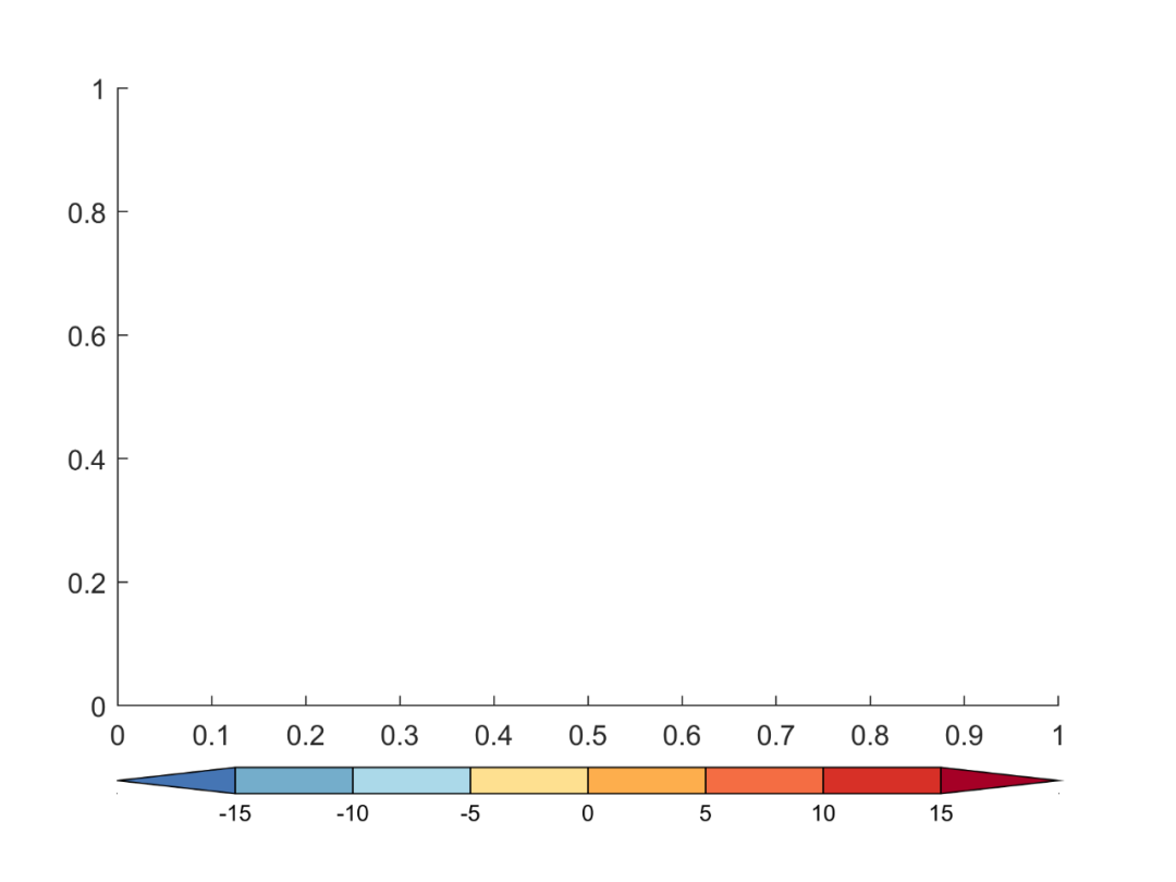

clc;clear;close allcolor=[131 0 162;160 0 198;109 0 219;31 60 249;0  160 230;0 198 198;0 209 139;0 219 0;160 230  51;230 219 51;230 175 45;239 130 41;239 0 0;219  0 98;255 1 118]/255;tick=515:5:590;mode='v';%----------------------------------------------------------data=importdata('fill_china.dat');lon=data(:,1);lat=data(:,2);data_9=[6 6];%lon lat data_9是绘图数据[ax1,c,h]=contf_line(lon,lat,data_9,tick,color,mode);set(gca,'fontname','Times New  Roman','fontsize',16,'fontangle','italic');set(c,'fontname','Times New Roman','fontsize',14)

function [ax1,c,h]=contf_line(lon,lat,X,tick,color,mode)% ---------------------------------%contourf()绘图，带尖端的colorbar%[ax1,c,h]=CONTF_LINE(lon,lat,X,tick,color,mode)% %tick的个数比color的行数多一个%ax1控制绘图窗，c控制colorbar,h控制contourf函数%--------%修改colorbar间隔：%lab=get(c,'x/yticklabel');%lab(2:2:end)={' '};%set(c,'x/yticklabel',lab);%--------%copyright 傅辉煌% ----------------------------------------[m,~]=size(color);len_tick=length(tick);if len_tick-m ~= 1    returnend[ax1,c]=colorbarn(tick,color,mode);[~,h]=contourf(lon,lat,X);set(h,'levellist',tick,'linecolor','none');colormap(color);caxis([tick(1) tick(end)])end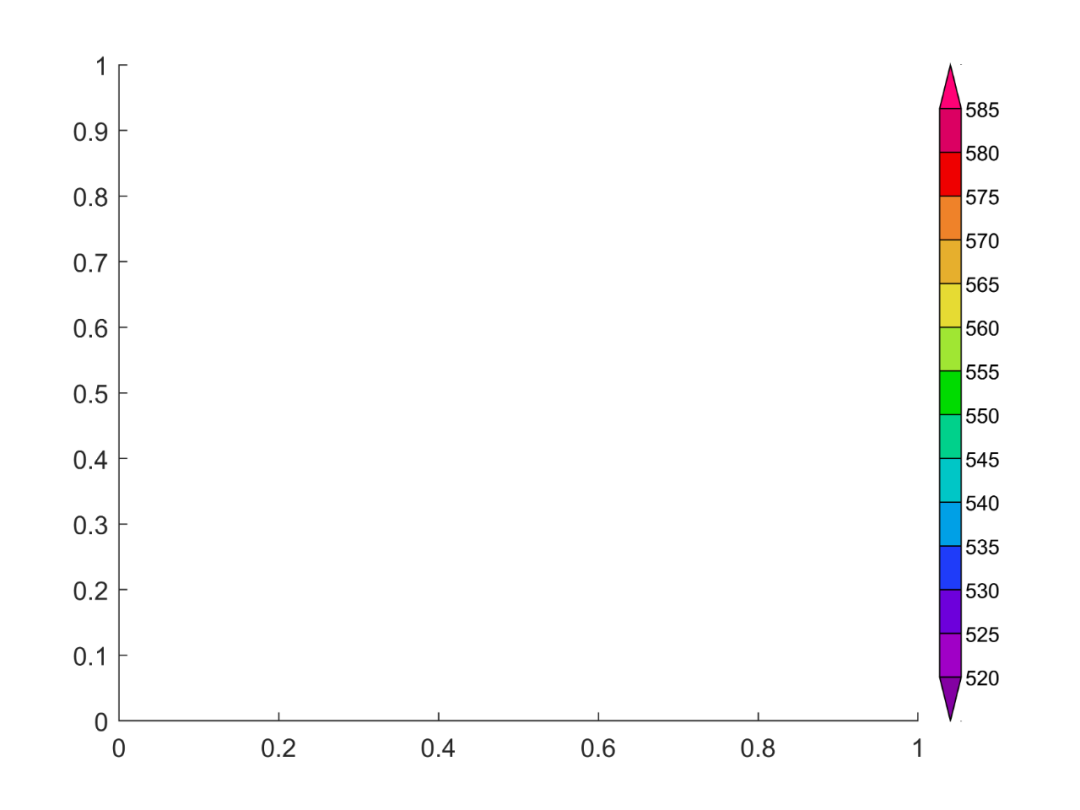

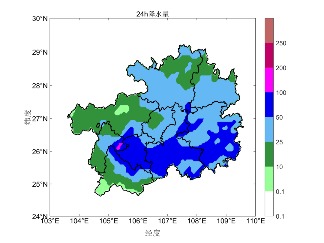
% 计算两个经纬度之间的距离% m_map工具箱里面的m_lldist% DIST=m_lldist([20 30],[44 45])clear all;close all;clcload('data.mat')load('map.mat');space_shp=0.05;xi=round(min(x_gz))-1:space_shp:round(max(x_gz))+1;yi=round(min(y_gz))-1:space_shp:round(max(y_gz))+1;[XI,YI]=meshgrid(xi,yi);ZI1=interp2(lon,lat,data,XI,YI,'nearest');    % 'linear'、'nearest'、'natural'、'cubic' 或 'v4'。默认方法为 'linear'isin=inpolygon(XI,YI,x_gz,y_gz);ZI1(~isin)=NaN;%% 降水量不等间距填色图% %降水量颜色设置cmap=[255 255 255; 150 255 150; 50 146 60; 100 184 244;...          0 0 241; 255 0 255; 192 0 100;192 100 100;]/255;level = [0.1,0.1,10,25,50,100,200,250] ;[~,ZI2]=histc(ZI1,level);ZI2=ZI2-1;%% 绘图figure('position',[50 50 800 600]);m_proj('mercator','lon',[103,110],'lat',[24,30]);[cs,h2]=m_contourf(XI,YI,ZI2,'LineWidth',1.5);  hold on  % --------------------------set(h2,'LineStyle','none');shading flat;           %填充平滑colormap(cmap) ;caxis([0 length(level)]) ;cbar = colorbar;set(cbar,'Ticks',0:length(level)-1,'TickLabels',level) ;set(cbar,'TickLength',0);m_plot(x_gz2,y_gz2,'LineWidth',1.5,'Color','k');set(gca,'FontSize',13);%m_grid('linest','none','tickdir','in');m_grid('box','fancy','tickdir','in');xlabel('经度');ylabel('纬度');title1=strcat('24h降水量');title(title1,'FontSize',13);% print('-dpng',strcat(title1,'.png'));hold off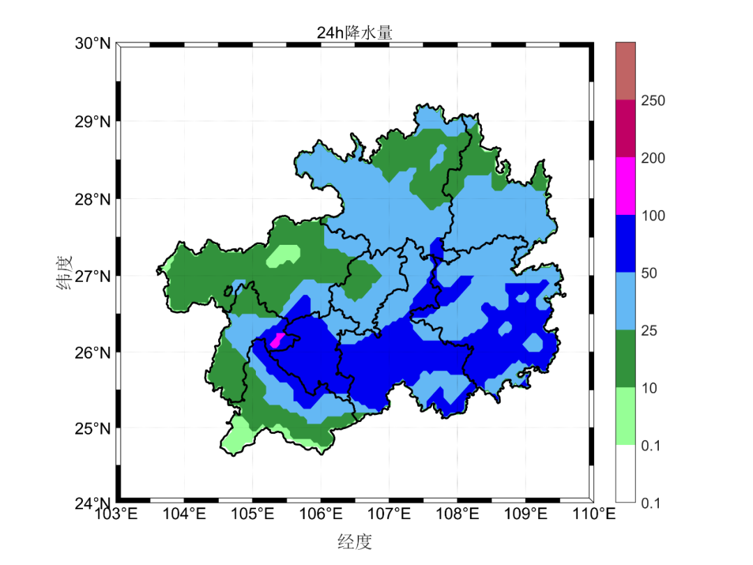

5 Plan

文章链接：Plan4