%Jacobian = [Jacobian_1_1 Jacobian_1_2;
% Jacobian_2_1 Jacobian_2_2;
% Jacobian_3_1 Jacobian_3_2;
% Jacobian_4_1 Jacobian_4_2;
% Jacobian_5_1 Jacobian_5_2];
[Jacobian_1_1,Jacobian_1_2] = func_Jacobian_1(Len_IVM,Num_Bus);
[Jacobian_2_1,Jacobian_2_2] = func_Jacobian_2(V_est,Ang_est,G,B,Index_real_power_injection,FROM_BUS,Len_IRPI,Num_Bus);
[Jacobian_3_1,Jacobian_3_2] = func_Jacobian_3(V_est,Ang_est,G,B,Index_reactive_power_injection,FROM_BUS,Len_IRP,Num_Bus);
[Jacobian_4_1,Jacobian_4_2] = func_Jacobian_4(V_est,Ang_est,G,B,Index_real_powerflow,FROM_BUS,TO_BUS,Len_IRPS,Num_Bus);
[Jacobian_5_1,Jacobian_5_2] = func_Jacobian_5(V_est,Ang_est,G,B,Shunt_Admittance,Index_reactive_powerflow,FROM_BUS,TO_BUS,Len_IRPF,Num_Bus);
% Measurement Jacobian, Jacobian..
Jacobian = [Jacobian_1_1 Jacobian_1_2;
Jacobian_2_1 Jacobian_2_2;
Jacobian_3_1 Jacobian_3_2;
Jacobian_4_1 Jacobian_4_2;
Jacobian_5_1 Jacobian_5_2];
Gm = Jacobian'*inv(Error)*Jacobian;
%计算误差
r = Values - h;
%进行状态估计
dE = inv(Gm)*(Jacobian'*inv(Error)*r);
Vector_est = Vector_est + Step*dE;
Ang_est(2:end) = Vector_est(1:Num_Bus-1);
V_est = Vector_est(Num_Bus:end);
Times = Times + 1;
Error_aim = mean(abs(dE));
errors(Times-1) = Error_aim;
h_est{Times-1} = h;
pause(0.001);
end
disp('状态估计结果');
disp('网络节点 --- 电压幅度 --- 电压相位角度');
for m = 1:Num_Bus
fprintf('%4d ',m);
fprintf('%8.8f ',V_est(m));
fprintf('%8.8f ',Ang_est(m));
fprintf('\n');
end
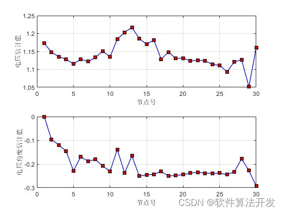
figure;
subplot(211);
plot(1:Num_Bus,V_est,'-bs',...
'LineWidth',1,...
'MarkerSize',6,...
'MarkerEdgeColor','k',...
'MarkerFaceColor',[0.9,0.0,0.0]);
grid on;
xlabel('节点号');
ylabel('电压估计值');
subplot(212);
plot(1:Num_Bus,Ang_est,'-bs',...
'LineWidth',1,...
'MarkerSize',6,...
'MarkerEdgeColor','k',...
'MarkerFaceColor',[0.9,0.0,0.0]);
grid on;
xlabel('节点号');
ylabel('电压角度估计值');
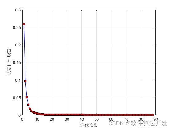
figure;
plot(errors,'-bs',...
'LineWidth',1,...
'MarkerSize',6,...
'MarkerEdgeColor','k',...
'MarkerFaceColor',[0.9,0.0,0.0]);
grid on;
xlabel('迭代次数');
ylabel('状态估计误差');
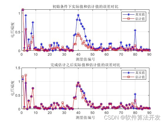
figure;
subplot(211);
plot(abs(Values),'b-*');
hold on
plot(abs(h_est{2}),'r-s');
grid on;
legend('真实值','估计值');
xlabel('测量值编号');
ylabel('电压幅度');
title('初始条件下实际值和估计值的误差对比');
subplot(212);
plot(abs(Values),'b-*');
hold on
plot(abs(h_est{end}),'r-s');
grid on;
legend('真实值','估计值');
xlabel('测量值编号');
ylabel('电压幅度');
title('完成估计之后实际值和估计值的误差对比');
27_004m
- 1.
- 2.
- 3.
- 4.
- 5.
- 6.
- 7.
- 8.
- 9.
- 10.
- 11.
- 12.
- 13.
- 14.
- 15.
- 16.
- 17.
- 18.
- 19.
- 20.
- 21.
- 22.
- 23.
- 24.
- 25.
- 26.
- 27.
- 28.
- 29.
- 30.
- 31.
- 32.
- 33.
- 34.
- 35.
- 36.
- 37.
- 38.
- 39.
- 40.
- 41.
- 42.
- 43.
- 44.
- 45.
- 46.
- 47.
- 48.
- 49.
- 50.
- 51.
- 52.
- 53.
- 54.
- 55.
- 56.
- 57.
- 58.
- 59.
- 60.
- 61.
- 62.
- 63.
- 64.
- 65.
- 66.
- 67.
- 68.
- 69.
- 70.
- 71.
- 72.
- 73.
- 74.
- 75.
- 76.
- 77.
- 78.
- 79.
- 80.
- 81.
- 82.
- 83.
- 84.
- 85.
- 86.
- 87.
- 88.
- 89.
- 90.
- 91.
- 92.
- 93.
- 94.
- 95.
- 96.
- 97.
- 98.
- 99.
- 100.
- 101.
- 102.


 1155
1155


 被折叠的 条评论
为什么被折叠?
被折叠的 条评论
为什么被折叠?
 到【灌水乐园】发言


