python 机器学习 爬取关键字_Python机器学习实战

前言

机器学习是从人工智能中产生的一个重要学科分支，是实现智能化的关键。其专门研究计算机怎样模拟或实现人类的学习行为，以获取新的知识或技能，重新组织已有的知识结构使之不断改善自身的性能。

目前机器学习主要使用Python完成，接下来本文将使用一个实例来讲解其具体应用。

1

模块介绍

sklearn是一个Python第三方提供的非常强力的机器学习库，它包含了从数据预处理到训练模型的各个方面。

在实战使用scikit-learn中可以极大的节省我们编写代码的时间以及减少我们的代码量，使我们有更多的精力去分析数据分布，调整模型和修改超参。

安装sklearn

scikit-learn需要：

Python(> = 2.7或> = 3.4)，

NumPy(> = 1.8.2)，

SciPy(> = 0.13.3)。

如果你已经安装了numpy和scipy，那么安装scikit-learn的最简单方法就是使用 pip或者canda：

pip install -U scikit-learnconda install scikit-learn

安装好sklearn之后，我们就可以用它来进行机器学习实战了。

2

算法介绍

机器学习中，决策树是一个预测模型；它代表的是对象属性与对象值之间的一种映射关系。

树中每个节点表示某个对象，而每个分叉路径则代表的某个可能的属性值，而每个叶结点则对应从根节点到该叶节点所经历的路径所表示的对象的值。

在sklearn库中，已经为我们准备好了决策树分类器，需要使用时直接导入即可。      

 from sklearn.tree import DecisionTreeClassifier

3

问题背景

鸢尾花，测量数据：花瓣的长度和宽度，花萼的长度和宽度，所有测量结果都以厘米为单位。

这一类花有三个品种：setosa, versicolor, virginnica。数据集中每朵鸢尾花叫做一个数据点，它的品种叫做它的标签。

在scikit-learn的datasets模块中，可以调用一些基础的训练数据集，其中之一就是load_iris函数，载入iris数据集，得到鸢尾花数据。

数据示例：

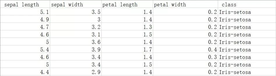
这是最基础的三分类问题，我们的目标是建立一个基础的机器学习的模型预测鸢尾花的品种。使用其sepal length, sepal width等属性来预测其可能属于的class。

4

实战代码

part1 数据集导入和处理

#导入数据from sklearn import datasetsimport numpy as npiris = datasets.load_iris()X = iris.data[:,[2,3]]#选择petal length和petal width两个属性Y = iris.targetprint(X)#随机选择训练集和测试集from sklearn.model_selection import train_test_splitX_train, X_test, Y_train, Y_test = train_test_split(X, Y, test_size=0.3, random_state=0)#数据标准化from sklearn.preprocessing import StandardScalersc = StandardScaler()sc.fit(X_train)X_train_std = sc.transform(X_train)X_test_std = sc.transform(X_test)

part2 数据集展示

print("类别标签:", np.unique(Y))print("总样本数量:", np.bincount(Y))print("训练集样本数量:", np.bincount(Y_train))print("测试集样本数量:", np.bincount(Y_test))

part3 训练决策树

from sklearn.tree import DecisionTreeClassifiertree = DecisionTreeClassifier(criterion='entropy', max_depth=3, random_state=0)tree.fit(X_train, Y_train)

part4 结果可视化

from matplotlib.colors import ListedColormapimport matplotlib.pyplot as pltdef plot_decision_regions(X, Y, classifier, test_idx=None, resolution=0.02):    markers = ('s','x','^','v','o')    colors = ('red','blue','lightgreen','gray','cyan')    cmap = ListedColormap(colors[:len(np.unique(Y))])    x1_min, x1_max = X[:, 0].min() - 1, X[:, 0].max() + 1    x2_min, x2_max = X[:, 1].min() - 1, X[:, 1].max() + 1    xx1, xx2 = np.meshgrid(np.arange(x1_min, x1_max, resolution), np.arange(x2_min, x2_max, resolution))    Z = classifier.predict(np.array([xx1.ravel(), xx2.ravel()]).T)    Z = Z.reshape(xx1.shape)    plt.contourf(xx1, xx2, Z, alpha=0.4, cmap=cmap)    plt.xlim(xx1.min(), xx1.max())    plt.ylim(xx2.min(), xx2.max())    X_test, Y_test = X[test_idx, :], Y[test_idx]    for idx, cl in enumerate(np.unique(Y)):        plt.scatter(x=X[Y == cl, 0], y=X[Y == cl, 1], alpha=0.8, c=colors[idx], marker=markers[idx],label=cl)    if test_idx:        X_test, Y_test = X[test_idx, :], Y[test_idx]        plt.scatter(X_test[:, 0], X_test[:, 1], c='', alpha=1.0, linewidth=1, marker='o', s=55, edgecolor='white', label='test set')return ZX_combined = np.vstack((X_train, X_test))Y_combined = np.hstack((Y_train, Y_test))result = plot_decision_regions(X_combined, Y_combined, classifier=tree, test_idx=range(105,150))plt.xlabel('petal length [cm]')plt.ylabel('petal width [cm]')plt.legend(loc='upper left')plt.show()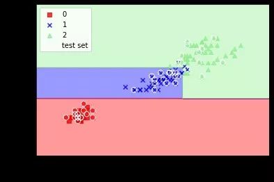

part5 评估模型

print("训练集的决定系数:",tree.score(X_train, Y_train))print("测试集的决定系数:",tree.score(X_test, Y_test))print("总样本的决定系数:",tree.score(X_combined, Y_combined))

part6 更进一步——随机森林

#集成多个弱分类器(单个决策树)形成不易过拟合的、有更小泛化误差的分类器from sklearn.ensemble import RandomForestClassifierforest = RandomForestClassifier(criterion='entropy', n_estimators=10, random_state=1, n_jobs=4)forest.fit(X_train, Y_train)plot_decision_regions(X_combined, Y_combined, classifier=forest, test_idx=range(105,150))plt.xlabel('petal length')plt.ylabel('petal width')plt.legend(loc='upper left')plt.show()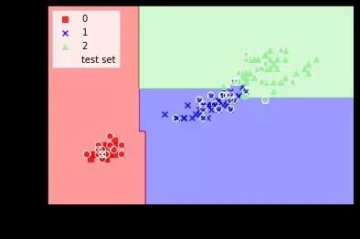

以上就是这期的全部内容了，希望能对大家有所帮助，也希望大家能够进行具体操作，付之实践。

本期作者：范人文

本期编辑校对：秦范

长按，关注数据皮皮侠