Atari 游戏训练 -- 2. 基于jupyter，图片处理 + state更新 + 经验回放数据初始化

帧图片处理 openCV

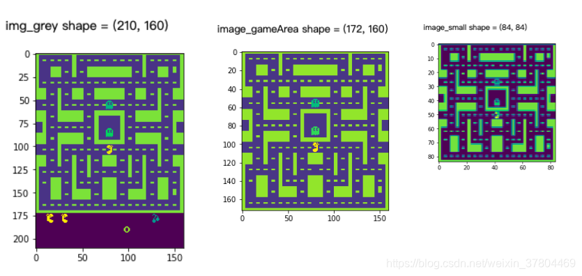
step1.图片灰度处理

图片灰度处理后，三通道（RGB） ===>> 单通道

两种方式：

1. 常用的公式对三通道进行处理：ray = R0.299 + G0.587 + B*0.114
2. openCV 直接灰度处理：img_grey=cv2.cvtColor(img,cv2.COLOR_BGR2GRAY)

step2.图片剪切，减去非游戏区域

step3.缩小图片至84*84

#别问我图片为什么不灰

import gym
import time
import cv2 
import torch
import torch.nn as nn
import numpy as np
import matplotlib.pyplot as plt         
import matplotlib.image as mpimg   


#chage the image size from 210*160*3 to 84*84
#change the RGB image into grey image

def preprocess(obs):
    img = obs.astype(np.float32)
    
    #step1: a common formula converting  converting RGB images into gray images: 
    #ray = R*0.299 + G*0.587 + B*0.114
    img_grey = img[:, :, 0] * 0.299 + img[:, :, 1] * 0.587 + img[:, :, 2] * 0.114  #shape = (210,160,1)  
    #img_grey=cv2.cvtColor(img,cv2.COLOR_BGR2GRAY)
    print('img_grey shape =', np.shape(img_grey))
    plt.imshow(img_grey) 
    plt.show()
    
    #step2: Crop out the non-game area of the image 
    image_gameArea = img_grey[0:172,:]      #shape = (172,160,1)  
    print('image_gameArea shape =', np.shape(image_gameArea))
    plt.imshow(image_gameArea) 
    plt.show()
    
    #step3: reduce the scale of the picture into 84*84
    image_small = cv2.resize(image_gameArea, (84, 84), interpolation=cv2.INTER_AREA)  # shape(84,84)
    print('image_small shape =', np.shape(image_small))
    plt.imshow(image_small) 
    plt.show()

---

state的初始化和迭代

设置定义：
observation：一帧图片
state： state是最近的、连续的4帧图片叠加。

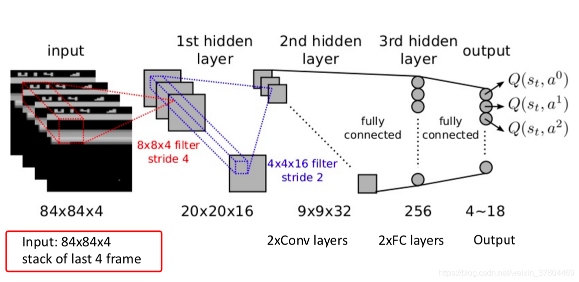
为什么要叠加4帧图片呢？因为有的游戏需要提取移动趋势特征，比如有两帧相同的图片（相同的observation），游戏角色在相同的位置，但是运动趋势不一样，一个是从左往右移动到这个位置，一个是从右往左移动到这个位置，提取游戏角色的移动趋势特征更有利于训练出准确的动作预测。

由上图可见，state会做为CNN的输入，经过多层卷集处理，输出是各个action对应的Q-value.后面文章会详细说明。

当刚加载游戏时，游戏处于第一帧图片时，这时自然是没有前3帧，怎么办呢？把这一帧图片复制4份叠加。

def init_state(self, obs):
        x = self.preprocess(obs) 
        state_initial = np.stack((x, x, x, x), axis=0)      # shape(4, 84, 84)      
        #print('shape_ state_initial  =', np.shape(state_initial)) 
        return state_initial

之后就不断迭代state：
在每做完一个动作后，会产生reward和next observation，把这个observation添加进state，然后最老的那个observation剔除出去，组成next state

    def next_state(self, state, obs):
        x = self.preprocess(obs)
        #state  = np.reshape(state, (4,84,84))
        next_state = np.append(state[1:, :, :], np.expand_dims(x, 0), axis=0)    # shape(4, 84, 84)
        #print('shape_next_state  =', np.shape(next_state))      
        return next_state

---

用于经验回放 的经验库的初始化 replay experience initialization

经验回放之后的文章会介绍，这里先说经验数据需要哪些字段
如果你学过Q-learning（Reinforcement Learning 的一种方式）, 你就会知道在其学习过程中，会需要： state, action, reward, next_state，这里也一样（就是多个个游戏是否结束的状态done）。

当然一样啦，因为经验回放就是用于Deep Q-learning Network 的学习的。

for epis in range(experience):        
    action = env.action_space.sample()
    obs, reward, done, _ = env.step(action)
    next_state = state_update(state,obs)          #shape_next_state  = (4, 84, 84)
    memory.append((state, action, reward, next_state, done))

---

附上完整代码，可以跑的那种

import gym
import time
import cv2 
import torch
import torch.nn as nn
import numpy as np
from collections import deque
import matplotlib.pyplot as plt         
import matplotlib.image as mpimg   


#chage the image size from 210*160*3 to 84*84
#change the RGB image into grey image

def preprocess(obs):
    img = obs.astype(np.float32)
    
    # a common formula converting  converting RGB images into gray images: ray = R*0.299 + G*0.587 + B*0.114
    img_grey = img[:, :, 0] * 0.299 + img[:, :, 1] * 0.587 + img[:, :, 2] * 0.114            #shape = (210,160,1)   
    #print('img_grey shape =', np.shape(img_grey))
    #plt.imshow(img_grey) 
    #plt.show()
    
    #Crop out the non-game area of the image 
    image_gameArea = resized_screen = img_grey[0:172,:]      #shape = (172,160,1)  
    #print('image_gameArea shape =', np.shape(image_gameArea))
    #plt.imshow(image_gameArea) 
    #plt.show()
    
    #reduce the scale of the picture into 84*84
    image_small = cv2.resize(image_gameArea, (84, 84), interpolation=cv2.INTER_AREA)   # shape(84,84)
    #print('image_small shape =', np.shape(image_small))
    #plt.imshow(image_small) 
    #plt.show()

    return image_small.astype(np.float32) / 255.0



def init_state(obs):
    x = preprocess(obs) 
    state_initial = np.stack((x, x, x, x), axis=0)      # shape(4, 84, 84)      
    #print('shape_ state_initial  =', np.shape(state_initial)) 
    return state_initial


def state_update(state, obs):
    x = preprocess(obs)
    #state  = np.reshape(state, (4,84,84))
    next_state = np.append(state[1:, :, :], np.expand_dims(x, 0), axis=0)    # shape(4, 84, 84)
    #print('shape_next_state  =', np.shape(next_state))      
    return next_state
    
    
    
experience = 1000  
memory = deque(maxlen=experience)    
env = gym.make('MsPacman-v0')
#print(env.observation_space)

obs = env.reset()  
state = init_state(obs)
#print('state  =', np.shape(state))
            
for epis in range(experience):        
    action = env.action_space.sample()
    obs, reward, done, _ = env.step(action)
    next_state = state_update(state,obs)          #shape_next_state  = (4, 84, 84)
    memory.append((state, action, reward, next_state, done))
        
        
    if done:
        print('done')
        obs = env.reset()               
        state = init_state(obs)             
    else:
        state = next_state
            
    time.sleep(0.05) # sleep for 1 second to observe the whole process
    env.render()      

env.close()