[Python深度学习]（五）深度学习用于文本和序列

最新推荐文章于 2023-05-10 11:26:50 发布

置顶 gdtop818

最新推荐文章于 2023-05-10 11:26:50 发布

阅读量1.9k

点赞数 3

本文链接：https://blog.csdn.net/weixin_37993251/article/details/85019703

版权

Python深度学习同时被 2 个专栏收录

7 篇文章 1 订阅

订阅专栏

Python深度学习——Deeplearning with Python

7 篇文章 21 订阅

订阅专栏

本文为《Python深度学习》的学习笔记。

第6章深度学习用于文本和序列

本章将使用深度学习模型处理文本、时间序列和一般的序列数据。

6.1 处理文本数据

深度学习模型不会接受原始文本作为输入，它只能处理数值张量。将文本分解成的单元叫做标记(token)，将文本分解成标记的过程叫做分词(tokenization)。本节介绍两种主要方法，对标记one-hot编码与标记嵌入（词嵌入word embedding）。
n-gram:是从一个句子中提取的N个连续单词的集合。比如“The cat sat on the mat.”可以分解为一下二元语法(2-grams)的集合。{"The","The cat", "cat", "cat sat", "sat",.....}
这样的集合叫做二元语法袋(bag-of-2-grams)。这里处理的是标记组成的集合，而不是一个列表或者序列。

6.1.1 单词和字符的one-hot编码

one-hot编码是将标记转换为向量的最常用、最基本的方法。

6-1 对每个单词进行one-hot编码
6-2 去掉一些特殊字符
6-3 设置只考虑前1000个常见单词
6-4 使用散列技巧的单词级的one-hot编码

# 6-1 单词级的one-hot编码
import numpy as np

# This is our initial data; one entry per "sample" 初始数据，每个样本是列表一个元素
# (in this toy example, a "sample" is just a sentence, but
# it could be an entire document).
samples = ['The cat sat on the mat.', 'The dog ate my homework.']

# First, build an index of all tokens in the data. 建立数据中所有标记的指引
token_index = {}
for sample in samples:
    # We simply tokenize the samples via the `split` method.
    # in real life, we would also strip punctuation and special characters
    # from the samples. 分割标点和特殊符号，用split方法
    for word in sample.split():
        if word not in token_index:
            # Assign a unique index to each unique word 
            token_index[word] = len(token_index) + 1
            # Note that we don't attribute index 0 to anything.

# Next, we vectorize our samples. 向量化数据

# We will only consider the first `max_length` words in each sample.
max_length = 10

# This is where we store our results:
results = np.zeros((len(samples), max_length, max(token_index.values()) + 1))
for i, sample in enumerate(samples):
    for j, word in list(enumerate(sample.split()))[:max_length]:
        index = token_index.get(word)
        results[i, j, index] = 1.

# 6-2 字符级的one-hot编码
import string

samples = ['The cat sat on the mat.', 'The dog ate my homework.']
characters = string.printable  # All printable ASCII characters. 打印所有的ascii码
token_index = dict(zip(characters, range(1, len(characters) + 1)))

max_length = 50
results = np.zeros((len(samples), max_length, max(token_index.values()) + 1))
for i, sample in enumerate(samples):
    for j, character in enumerate(sample[:max_length]):
        index = token_index.get(character)
        results[i, j, index] = 1.

# 6-3 用keras实现单词级的one-hot编码
from keras.preprocessing.text import Tokenizer

samples = ['The cat sat on the mat.', 'The dog ate my homework.']

# We create a tokenizer, configured to only take
# into account the top-1000 most common words
tokenizer = Tokenizer(num_words=1000)
# This builds the word index
tokenizer.fit_on_texts(samples)

# This turns strings into lists of integer indices.
sequences = tokenizer.texts_to_sequences(samples)

# You could also directly get the one-hot binary representations.
# Note that other vectorization modes than one-hot encoding are supported!
one_hot_results = tokenizer.texts_to_matrix(samples, mode='binary')

# This is how you can recover the word index that was computed
word_index = tokenizer.word_index
print('Found %s unique tokens.' % len(word_index))

# 6-4 使用散列技巧的单词级的One-hot编码
samples = ['The cat sat on the mat.', 'The dog ate my homework.']

# We will store our words as vectors of size 1000.
# Note that if you have close to 1000 words (or more)
# you will start seeing many hash collisions, which
# will decrease the accuracy of this encoding method.
dimensionality = 1000
max_length = 10

results = np.zeros((len(samples), max_length, dimensionality))
for i, sample in enumerate(samples):
    for j, word in list(enumerate(sample.split()))[:max_length]:
        # Hash the word into a "random" integer index
        # that is between 0 and 1000
        index = abs(hash(word)) % dimensionality
        results[i, j, index] = 1.

这里介绍以下tokenizer的用法：

科学使用Tokenizer的方法是，首先用Tokenizer的 fit_on_texts 方法学习出文本的字典，然后word_index 就是对应的单词和数字的映射关系dict
通过这个dict可以将每个string的每个词转成数字，可以用texts_to_sequences，这是我们需要的，然后通过padding的方法补成同样长度，在用keras中自带的embedding层进行一个向量化，并输入到LSTM中。

参考：如何科学地使用keras的Tokenizer进行文本预处理

from keras.preprocessing.text import Tokenizer

somestr = ['ha ha gua angry','howa ha gua excited naive']
tok = Tokenizer()
tok.fit_on_texts(somestr)
tok.word_index
Out[90]: {'angry': 3, 'excited': 5, 'gua': 2, 'ha': 1, 'howa': 4, 'naive': 6}
tok.texts_to_sequences(somestr)
Out[91]: [[1, 1, 2, 3], [4, 1, 2, 5, 6]]

6.1.2 使用词嵌入

word embedding
密集、低维、从数据学习中得到

1.利用Embedding层学习词嵌入：将一个词与一个密集向量相关联，最简单的方法是随机选择变量

# 6-5 将一个Embedding层实例化
from keras.layers import Embedding

# The Embedding layer takes at least two arguments:
# the number of possible tokens, here 1000 (1 + maximum word index),
# and the dimensionality of the embeddings, here 64.
embedding_layer = Embedding(1000, 64)

Embedding层接受整数作为输入，并在内部字典中查找这些数字，并返回相关联的变量。输入为二位整数张量，形状为（samples, sequence_length），返回一个三维浮点数张量（samples, sequence_length，dimensionality）。这里应用于IMDB电影评论情感预测人物。将电影评论限制为钱10000个常见的单词，再讲评论长度限制只有20个单词。

# 6-6 加载IMDB数据，准备用于Embedding层
from keras.datasets import imdb
from keras import preprocessing

# Number of words to consider as features
max_features = 10000
# Cut texts after this number of words 
# (among top max_features most common words)
maxlen = 20

# Load the data as lists of integers.
(x_train, y_train), (x_test, y_test) = imdb.load_data(num_words=max_features)

# This turns our lists of integers
# into a 2D integer tensor of shape `(samples, maxlen)`
x_train = preprocessing.sequence.pad_sequences(x_train, maxlen=maxlen)
x_test = preprocessing.sequence.pad_sequences(x_test, maxlen=maxlen)

# 6-7 在IMDB数据上使用Embedding层和分类器
from keras.models import Sequential
from keras.layers import Flatten, Dense

model = Sequential()
# We specify the maximum input length to our Embedding layer
# so we can later flatten the embedded inputs
model.add(Embedding(10000, 8, input_length=maxlen))
# After the Embedding layer, 
# our activations have shape `(samples, maxlen, 8)`.

# We flatten the 3D tensor of embeddings 
# into a 2D tensor of shape `(samples, maxlen * 8)`
model.add(Flatten())

# We add the classifier on top
model.add(Dense(1, activation='sigmoid'))
model.compile(optimizer='rmsprop', loss='binary_crossentropy', metrics=['acc'])
model.summary()

history = model.fit(x_train, y_train,
                    epochs=10,
                    batch_size=32,
                    validation_split=0.2)

2. 使用预训练的词嵌入
kearas模型中word2vec嵌入，案例见下面从imdb获取原始文本使用预训练GloVe的词嵌入模型。

6.1.3 整合在一起：从原始文本到词嵌入

1. 下载IMDB数据的原始文本: http://mng.bz/0tIo

# 6-8 处理IMDB原始数据的标签

import os

imdb_dir = 'C:/Users/adward/Desktop/deeplearning_with_python/aclImdb'
train_dir = os.path.join(imdb_dir, 'train')

labels = []
texts = []

for label_type in ['neg', 'pos']:
    dir_name = os.path.join(train_dir, label_type)
    for fname in os.listdir(dir_name):
        if fname[-4:] == '.txt':
            f = open(os.path.join(dir_name, fname),encoding='UTF-8')
            texts.append(f.read())
            f.close()
            if label_type == 'neg':
                labels.append(0)
            else:
                labels.append(1)

2.对数据进行分词
划分为训练集和验证集。将训练数据限定为前200个样本，在读取了前200个样本后学习对电影评论分类。

# 6-9 对IMDB原始数据的文本进行分词

from keras.preprocessing.text import Tokenizer
from keras.preprocessing.sequence import pad_sequences
import numpy as np

maxlen = 100  # We will cut reviews after 100 words
training_samples = 200  # We will be training on 200 samples
validation_samples = 10000  # We will be validating on 10000 samples
max_words = 10000  # We will only consider the top 10,000 words in the dataset

tokenizer = Tokenizer(num_words=max_words)
tokenizer.fit_on_texts(texts)
sequences = tokenizer.texts_to_sequences(texts)

word_index = tokenizer.word_index
print('Found %s unique tokens.' % len(word_index))

data = pad_sequences(sequences, maxlen=maxlen)

labels = np.asarray(labels)
print('Shape of data tensor:', data.shape)
print('Shape of label tensor:', labels.shape)

# Split the data into a training set and a validation set
# But first, shuffle the data, since we started from data
# where sample are ordered (all negative first, then all positive).
indices = np.arange(data.shape[0])
np.random.shuffle(indices)
data = data[indices]
labels = labels[indices]

x_train = data[:training_samples]
y_train = labels[:training_samples]
x_val = data[training_samples: training_samples + validation_samples]
y_val = labels[training_samples: training_samples + validation_samples]

Found 88582 unique tokens.
Shape of data tensor: (25000, 100)
Shape of label tensor: (25000,)

代码中一些注意地方：

np.asarray(a, dtype=None, order=None) —— 将结构数据转化为ndarray。
np.arange()函数返回一个有终点和起点的固定步长的排列

参数个数情况： np.arange()函数分为一个参数，两个参数，三个参数三种情况
1）一个参数时，参数值为终点，起点取默认值0，步长取默认值1。
2）两个参数时，第一个参数为起点，第二个参数为终点，步长取默认值1。
3）三个参数时，第一个参数为起点，第二个参数为终点，第三个参数为步长。其中步长支持小数。
np.arange函数

3.下载GloVe词嵌入 http://nlp.stanford.edu/data/glove.6B.zip（2014年英文维基百科的预计算嵌入）

包含400000个单词的100维嵌入向量

4.对嵌入进行预处理

# 6-10 解析Glove词嵌入文件

glove_dir = 'C:/Users/adward/Desktop/deeplearning_with_python'

embeddings_index = {}
f = open(os.path.join(glove_dir, 'glove.6B.100d.txt'), encoding = 'UTF-8')
for line in f:
    values = line.split()
    word = values[0]
    coefs = np.asarray(values[1:], dtype='float32')
    embeddings_index[word] = coefs
f.close()

print('Found %s word vectors.' % len(embeddings_index))

Found 400000 word vectors.

接下来构建一个可以加载到Embedding层中的嵌入矩阵embedding_matrix。

# 6-11 准备GloVe词嵌入矩阵

embedding_dim = 100

embedding_matrix = np.zeros((max_words, embedding_dim))
for word, i in word_index.items():
    if i < max_words:
        embedding_vector = embeddings_index.get(word)
        if(embedding_vector is not None):
            embedding_matrix[i] = embedding_vector

5.定义模型
使用与前面相同的模型架构

# 6-12 模型定义
from keras.models import Sequential
from keras.layers import Embedding, Flatten, Dense

model = Sequential()
model.add(Embedding(max_words, embedding_dim, input_length=maxlen))
model.add(Flatten())
model.add(Dense(32, activation='relu'))
model.add(Dense(1, activation='sigmoid'))
model.summary()

6.在模型中加载Glove嵌入

此时需要冻结Embedding层，英文这一部分模型是经过了预训练的，那么在训练期间不会更新预训练部分。

# 6-13 将预训练的词嵌入加载到Embedding层中
model.layers[0].set_weights([embedding_matrix])
model.layers[0].trainable = False

7.训练模型与评估模型（使用预训练的词嵌入）

# 6-14 训练与评估
model.compile(optimizer='rmsprop',
              loss='binary_crossentropy',
              metrics=['acc'])
history = model.fit(x_train, y_train,
                    epochs=10,
                    batch_size=32,
                    validation_data=(x_val, y_val))
model.save_weights('pre_trained_glove_model.h5')

# 6-15 绘制结果
import matplotlib.pyplot as plt

acc = history.history['acc']
val_acc = history.history['val_acc']
loss = history.history['loss']
val_loss = history.history['val_loss']

epochs = range(1, len(acc) + 1)

plt.plot(epochs, acc, 'bo', label='Training acc')
plt.plot(epochs, val_acc, 'b', label='Validation acc')
plt.title('Training and validation accuracy')
plt.legend()

plt.figure()

plt.plot(epochs, loss, 'bo', label='Training loss')
plt.plot(epochs, val_loss, 'b', label='Validation loss')
plt.title('Training and validation loss')
plt.legend()

plt.show()

我们发现训练样本很少，模型很快就过拟合了，并且验证精度波动很大。

这里我们和不使用预训练词嵌入情况下训练相同模型。

# 6-16 在不使用预训练词嵌入情况下，训练相同模型
from keras.models import Sequential
from keras.layers import Embedding, Flatten, Dense

model = Sequential()
model.add(Embedding(max_words, embedding_dim, input_length=maxlen))
model.add(Flatten())
model.add(Dense(32, activation='relu'))
model.add(Dense(1, activation='sigmoid'))
model.summary()

model.compile(optimizer='rmsprop',
              loss='binary_crossentropy',
              metrics=['acc'])
history = model.fit(x_train, y_train,
                    epochs=10,
                    batch_size=32,
                    validation_data=(x_val, y_val))

绘制图形：

预训练词嵌入的性能要优于与任务一起学习的嵌入。

这里发现预训练词嵌入的性能要优于与任务一起学习的嵌入。最后在测试数据上评估。

# 6-17 对测试数据进行分词
test_dir = os.path.join(imdb_dir, 'test')

labels = []
texts = []

for label_type in ['neg', 'pos']:
    dir_name = os.path.join(test_dir, label_type)
    for fname in sorted(os.listdir(dir_name)):
        if fname[-4:] == '.txt':
            f = open(os.path.join(dir_name, fname), encoding = 'UTF-8')
            texts.append(f.read())
            f.close()
            if label_type == 'neg':
                labels.append(0)
            else:
                labels.append(1)

sequences = tokenizer.texts_to_sequences(texts)
x_test = pad_sequences(sequences, maxlen=maxlen)
y_test = np.asarray(labels)

# 6-18 在测试集上评估模型
model.load_weights('pre_trained_glove_model.h5')
model.evaluate(x_test, y_test)

25000/25000 [==============================] - 2s 86us/step

[0.7450807450962067, 0.57592]

可以看到我们仅仅使用了很少的训练样本，但是准确率达到了57%！

6.1.4 小结

将原始文本转换为神经网络能处理的格式
使用Keras模型的Embedding层来学习针对特定任务的标记嵌入
使用预训练词嵌入在小型自然语言处理问题上获得额外的性能提升

6.2 理解循环神经网络

原理在我另外一篇文章详细介绍[实战Google深度学习框架]Tensorflow(7)自然语言处理

# 6-19 RNN伪代码
state_t = 0 
for input_t in input_sequence:
    output_t = f(input_t, state_t)
    state_t = output_t

# 6-20 更详细的RNN伪代码
state_t = 0 
for input_t in input_sequence:
    output_t = activation(dot(W, input_t) + dot(U, state_t) + b)
    state_t = output_t

下面我们用简单的RNN前向传播编写一个网络

# 6-21 简单RNN的Numpy实现
import numpy as np

timesteps = 100 # 输入序列的时间步数
input_features = 32 # 输入特征空间的维度
output_features = 64 # 输出特征空间的维度

inputs = np.random.random((timesteps, input_features))

state_t = np.zeros((output_features,))

W = np.random.random((output_features, input_features))
U = np.random.random((output_features, output_features))
b = np.random.random((output_features,))

successive_outputs = []
for input_t in inputs:
    output_t = np.tanh(np.dot(W, input_t) + np.dot(U, state_t) + b)
    
    successive_outputs.append(output_t)
    
    state_t = output_t
    
final_output_sequence = np.stack(successive_outputs, axis = 0)

6.2.1 Keras中的循环层

这里的SimpleRNN层和其他Keras层一样处理序列批量，SimpleRNN可以在两种不同的模式下运行：

返回每个时间步连续输出的完整序列
只返回每个输入序列的最终输出

from keras.layers import SimpleRNN

from keras.models import Sequential
from keras.layers import Embedding, SimpleRNN

model = Sequential()
model.add(Embedding(10000, 32))
model.add(SimpleRNN(32))
model.summary()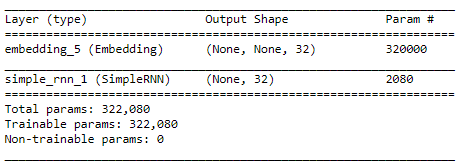

下面这个模型返回完整的状态序列。return_sequences=True

model = Sequential()
model.add(Embedding(10000, 32))
model.add(SimpleRNN(32, return_sequences=True))
model.summary()

为了提高网络的表示能力，将多个循环层堆叠起来、需要让所有中间层都返回完整输出序列。return_sequences=True

model = Sequential()
model.add(Embedding(10000, 32))
model.add(SimpleRNN(32, return_sequences=True))
model.add(SimpleRNN(32, return_sequences=True))
model.add(SimpleRNN(32, return_sequences=True))
model.add(SimpleRNN(32))  # This last layer only returns the last outputs.
model.summary()

下面，将这个模型应用于IMDB电影评论分类问题。首先，数据预处理

# 6-22 准备IMDB数据
from keras.datasets import imdb
from keras.preprocessing import sequence

max_features = 10000  # number of words to consider as features
maxlen = 500  # cut texts after this number of words (among top max_features most common words)
batch_size = 32

print('Loading data...')
(input_train, y_train), (input_test, y_test) = imdb.load_data(num_words=max_features)
print(len(input_train), 'train sequences')
print(len(input_test), 'test sequences')

print('Pad sequences (samples x time)')
input_train = sequence.pad_sequences(input_train, maxlen=maxlen)
input_test = sequence.pad_sequences(input_test, maxlen=maxlen)
print('input_train shape:', input_train.shape)
print('input_test shape:', input_test.shape)

Loading data...
25000 train sequences
25000 test sequences
Pad sequences (samples x time)
input_train shape: (25000, 500)
input_test shape: (25000, 500)

用一个Embedding层和SimpleRNN层来训练模型

# 6-23 用Embedding层和SimpleRNN层来训练模型
from keras.layers import Dense

model = Sequential()
model.add(Embedding(max_features, 32))
model.add(SimpleRNN(32))
model.add(Dense(1, activation='sigmoid'))

model.compile(optimizer='rmsprop', loss='binary_crossentropy', metrics=['acc'])
history = model.fit(input_train, y_train,
                    epochs=10,
                    batch_size=128,
                    validation_split=0.2)

# 6-24 绘制结果
import matplotlib.pyplot as plt

acc = history.history['acc']
val_acc = history.history['val_acc']
loss = history.history['loss']
val_loss = history.history['val_loss']

epochs = range(len(acc))

plt.plot(epochs, acc, 'bo', label='Training acc')
plt.plot(epochs, val_acc, 'b', label='Validation acc')
plt.title('Training and validation accuracy')
plt.legend()

plt.figure()

plt.plot(epochs, loss, 'bo', label='Training loss')
plt.plot(epochs, val_loss, 'b', label='Validation loss')
plt.title('Training and validation loss')
plt.legend()

plt.show()

这里验证精度只有85%，问题在于只考虑了前500个单词，而不是整个序列。SImpleRNN不适合处理长序列

6.2.2 理解LSTM层和GRU层

LSTM精妙之处在于携带数据流下一个值的计算方法。

# 6-25 LSTM架构的详细伪代码(1/2)
output_t = activation(dot(state_t, Uo) + dot(input_t, Wo) + dot(C_t, Vo) + bo)

i_t = activation(dot(state_t, Ui) + dot(input_t, Wi) + bi)
f_t = activation(dot(state_t, Uf) + dot(input_t, Wf) + bf)
k_t = activation(dot(state_t, Uk) + dot(input_t, Wk) + bk)

# 6-26 LSTM架构的详细伪代码(2/2)
c_t+1 = i_t * k_t + c_t * f_t

6.2.3 Keras中一个LSTM的具体例子

# 6-27 使用Keras中的LSTM层
from keras.layers import LSTM

model = Sequential()
model.add(Embedding(max_features, 32))
model.add(LSTM(32))
model.add(Dense(1, activation='sigmoid'))

model.compile(optimizer='rmsprop',
              loss='binary_crossentropy',
              metrics=['acc'])
history = model.fit(input_train, y_train,
                    epochs=10,
                    batch_size=128,
                    validation_split=0.2)

acc = history.history['acc']
val_acc = history.history['val_acc']
loss = history.history['loss']
val_loss = history.history['val_loss']

epochs = range(len(acc))

plt.plot(epochs, acc, 'bo', label='Training acc')
plt.plot(epochs, val_acc, 'b', label='Validation acc')
plt.title('Training and validation accuracy')
plt.legend()

plt.figure()

plt.plot(epochs, loss, 'bo', label='Training loss')
plt.plot(epochs, val_loss, 'b', label='Validation loss')
plt.title('Training and validation loss')
plt.legend()

plt.show()

这一次，验证精度达到了89%，因为LSTM受梯度消失的问题影响会很小。

6.3 循环神经网络的高级用法

主要介绍以下三种技巧：

循环dropout（recurrent dropout）
堆叠循环层（stacking recurrent layers）
双向循环层（bidirectional recurrent layer）

6.3.1 温度预测问题

https://s3.amazonaws.com/keras-datasets/jena_climate_2009_2016.csv.zip

# 6-28 观察耶拿天气数据集的数据
import os

data_dir = 'C:/Users/adward/Desktop/deeplearning_with_python/'
fname = os.path.join(data_dir, 'jena_climate_2009_2016.csv')

f = open(fname)
data = f.read()
f.close()

lines = data.split('\n')
header = lines[0].split(',')
lines = lines[1:]

print(header)
print(len(lines))

['"Date Time"', '"p (mbar)"', '"T (degC)"', '"Tpot (K)"', '"Tdew (degC)"', '"rh (%)"', '"VPmax (mbar)"', '"VPact (mbar)"', '"VPdef (mbar)"', '"sh (g/kg)"', '"H2OC (mmol/mol)"', '"rho (g/m**3)"', '"wv (m/s)"', '"max. wv (m/s)"', '"wd (deg)"']
420551

# 6-29 解析数据
import numpy as np

float_data = np.zeros((len(lines), len(header) - 1))
for i, line in enumerate(lines):
    values = [float(x) for x in line.split(',')[1:]]
    float_data[i, :] = values

# 6-30 绘制温度时间序列
from matplotlib import pyplot as plt

temp = float_data[:, 1]  # temperature (in degrees Celsius)
plt.plot(range(len(temp)), temp)
plt.show()

# 6-31 绘制前10天的温度时间序列
plt.plot(range(1440), temp[:1440])
plt.show()

6.3.2 准备数据

lookback = 720: 给定过去5天内的观测数据

steps = 6：观测数据的采样频率是每小时一个数据点

delay = 144：目标是未来24小时之后的数据

# 6-32 数据标准化
mean = float_data[:200000].mean(axis=0)
float_data -= mean
std = float_data[:200000].std(axis=0)
float_data /= std

# 6-33 生成时间序列样本及其目标的生成器
def generator(data, lookback, delay, min_index, max_index,
              shuffle=False, batch_size=128, step=6):
    if max_index is None:
        max_index = len(data) - delay - 1
    i = min_index + lookback
    while 1:
        if shuffle:
            rows = np.random.randint(
                min_index + lookback, max_index, size=batch_size)
        else:
            if i + batch_size >= max_index:
                i = min_index + lookback
            rows = np.arange(i, min(i + batch_size, max_index))
            i += len(rows)

        samples = np.zeros((len(rows),
                           lookback // step,
                           data.shape[-1]))
        targets = np.zeros((len(rows),))
        for j, row in enumerate(rows):
            indices = range(rows[j] - lookback, rows[j], step)
            samples[j] = data[indices]
            targets[j] = data[rows[j] + delay][1]
        yield samples, targets

使用这个抽象的generator函数来实例化三个生成器。

# 6-34 准备训练生成器、验证生成器和测试生成器
lookback = 1440
step = 6
delay = 144
batch_size = 128

train_gen = generator(float_data,
                      lookback=lookback,
                      delay=delay,
                      min_index=0,
                      max_index=200000,
                      shuffle=True,
                      step=step, 
                      batch_size=batch_size)
val_gen = generator(float_data,
                    lookback=lookback,
                    delay=delay,
                    min_index=200001,
                    max_index=300000,
                    step=step,
                    batch_size=batch_size)
test_gen = generator(float_data,
                     lookback=lookback,
                     delay=delay,
                     min_index=300001,
                     max_index=None,
                     step=step,
                     batch_size=batch_size)

# This is how many steps to draw from `val_gen`
# in order to see the whole validation set:
val_steps = (300000 - 200001 - lookback) // batch_size

# This is how many steps to draw from `test_gen`
# in order to see the whole test set:
test_steps = (len(float_data) - 300001 - lookback) // batch_size

# 计算符合常识的基准方法
def evaluate_naive_method():
    batch_maes = []
    for step in range(val_steps):
        samples, targets = next(val_gen)
        preds = samples[:, -1, 1]
        mae = np.mean(np.abs(preds - targets))
        batch_maes.append(mae)
    print(np.mean(batch_maes))
    
evaluate_naive_method()

0.2897359729905486

# 6-36 jian将MAE转换成摄氏温度误差
celsius_mae = 0.29 * std[1]

6.3.3 一种基于常识的、非机器学习的基准方法

# 6-37 训练并评估一个密集连接模型
from keras.models import Sequential
from keras import layers
from keras.optimizers import RMSprop

model = Sequential()
model.add(layers.Flatten(input_shape=(lookback // step, float_data.shape[-1])))
model.add(layers.Dense(32, activation='relu'))
model.add(layers.Dense(1))

model.compile(optimizer=RMSprop(), loss='mae')
history = model.fit_generator(train_gen,
                              steps_per_epoch=500,
                              epochs=20,
                              validation_data=val_gen,
                              validation_steps=val_steps)

# 6-38 绘制结果
import matplotlib.pyplot as plt

loss = history.history['loss']
val_loss = history.history['val_loss']

epochs = range(len(loss))

plt.figure()

plt.plot(epochs, loss, 'bo', label='Training loss')
plt.plot(epochs, val_loss, 'b', label='Validation loss')
plt.title('Training and validation loss')
plt.legend()

plt.show()

寻找特定类型的简单模型。

6.3.5 第一个循环网络基准

GRU层，计算代价比LSTM更低。

# 6-39 训练并评估一个基于GRU的模型
from keras.models import Sequential
from keras import layers
from keras.optimizers import RMSprop

model = Sequential()
model.add(layers.GRU(32, input_shape=(None, float_data.shape[-1])))
model.add(layers.Dense(1))

model.compile(optimizer=RMSprop(), loss='mae')
history = model.fit_generator(train_gen,
                              steps_per_epoch=500,
                              epochs=20,
                              validation_data=val_gen,
                              validation_steps=val_steps)

loss = history.history['loss']
val_loss = history.history['val_loss']

epochs = range(len(loss))

plt.figure()

plt.plot(epochs, loss, 'bo', label='Training loss')
plt.plot(epochs, val_loss, 'b', label='Validation loss')
plt.title('Training and validation loss')
plt.legend()

plt.show()

新的MAE约为0.265。

6.3.6 使用循环dropout来降低过拟合

使用dropout正则化的网络总是需要更长的时间才能完全收敛。

# 6-40 训练并评估一个使用dropout正则化的基于GRU的模型
from keras.models import Sequential
from keras import layers
from keras.optimizers import RMSprop

model = Sequential()
model.add(layers.GRU(32,
                     dropout=0.2,
                     recurrent_dropout=0.2,
                     input_shape=(None, float_data.shape[-1])))
model.add(layers.Dense(1))

model.compile(optimizer=RMSprop(), loss='mae')
history = model.fit_generator(train_gen,
                              steps_per_epoch=500,
                              epochs=40,
                              validation_data=val_gen,
                              validation_steps=val_steps)

loss = history.history['loss']
val_loss = history.history['val_loss']

epochs = range(len(loss))

plt.figure()

plt.plot(epochs, loss, 'bo', label='Training loss')
plt.plot(epochs, val_loss, 'b', label='Validation loss')
plt.title('Training and validation loss')
plt.legend()

plt.show()

6.3.7 循环层堆叠

堆叠循环层，所有的中间层都一个返回完整的输出序列。return_sequences = True

# 6-41 训练并评估一个使用dropout正则化的堆叠GRU模型
from keras.models import Sequential
from keras import layers
from keras.optimizers import RMSprop

model = Sequential()
model.add(layers.GRU(32,
                     dropout=0.1,
                     recurrent_dropout=0.5,
                     return_sequences=True,
                     input_shape=(None, float_data.shape[-1])))
model.add(layers.GRU(64, activation='relu',
                     dropout=0.1, 
                     recurrent_dropout=0.5))
model.add(layers.Dense(1))

model.compile(optimizer=RMSprop(), loss='mae')
history = model.fit_generator(train_gen,
                              steps_per_epoch=500,
                              epochs=40,
                              validation_data=val_gen,
                              validation_steps=val_steps)

loss = history.history['loss']
val_loss = history.history['val_loss']

epochs = range(len(loss))

plt.figure()

plt.plot(epochs, loss, 'bo', label='Training loss')
plt.plot(epochs, val_loss, 'b', label='Validation loss')
plt.title('Training and validation loss')
plt.legend()

plt.show()

6.3.8 使用双向RNN

def reverse_order_generator(data, lookback, delay, min_index, max_index,
                            shuffle=False, batch_size=128, step=6):
    if max_index is None:
        max_index = len(data) - delay - 1
    i = min_index + lookback
    while 1:
        if shuffle:
            rows = np.random.randint(
                min_index + lookback, max_index, size=batch_size)
        else:
            if i + batch_size >= max_index:
                i = min_index + lookback
            rows = np.arange(i, min(i + batch_size, max_index))
            i += len(rows)

        samples = np.zeros((len(rows),
                           lookback // step,
                           data.shape[-1]))
        targets = np.zeros((len(rows),))
        for j, row in enumerate(rows):
            indices = range(rows[j] - lookback, rows[j], step)
            samples[j] = data[indices]
            targets[j] = data[rows[j] + delay][1]
        yield samples[:, ::-1, :], targets
        
train_gen_reverse = reverse_order_generator(
    float_data,
    lookback=lookback,
    delay=delay,
    min_index=0,
    max_index=200000,
    shuffle=True,
    step=step, 
    batch_size=batch_size)
val_gen_reverse = reverse_order_generator(
    float_data,
    lookback=lookback,
    delay=delay,
    min_index=200001,
    max_index=300000,
    step=step,
    batch_size=batch_size)

model = Sequential()
model.add(layers.GRU(32, input_shape=(None, float_data.shape[-1])))
model.add(layers.Dense(1))

model.compile(optimizer=RMSprop(), loss='mae')
history = model.fit_generator(train_gen_reverse,
                              steps_per_epoch=500,
                              epochs=20,
                              validation_data=val_gen_reverse,
                              validation_steps=val_steps)

loss = history.history['loss']
val_loss = history.history['val_loss']

epochs = range(len(loss))

plt.figure()

plt.plot(epochs, loss, 'bo', label='Training loss')
plt.plot(epochs, val_loss, 'b', label='Validation loss')
plt.title('Training and validation loss')
plt.legend()

plt.show()

双向RNN在某些数据上比普通RNN更好，逆序GRU的效果甚至比基于常识的基准方法还要差很多。

# 6-42 使用逆序序列序列并评估一个LSTM
from keras.datasets import imdb
from keras.preprocessing import sequence
from keras import layers
from keras.models import Sequential

# Number of words to consider as features
max_features = 10000
# Cut texts after this number of words (among top max_features most common words)
maxlen = 500

# Load data
(x_train, y_train), (x_test, y_test) = imdb.load_data(num_words=max_features)

# Reverse sequences
x_train = [x[::-1] for x in x_train]
x_test = [x[::-1] for x in x_test]

# Pad sequences
x_train = sequence.pad_sequences(x_train, maxlen=maxlen)
x_test = sequence.pad_sequences(x_test, maxlen=maxlen)

model = Sequential()
model.add(layers.Embedding(max_features, 128))
model.add(layers.LSTM(32))
model.add(layers.Dense(1, activation='sigmoid'))

model.compile(optimizer='rmsprop',
              loss='binary_crossentropy',
              metrics=['acc'])
history = model.fit(x_train, y_train,
                    epochs=10,
                    batch_size=128,
                    validation_split=0.2)

逆序处理效果和正序处理一样好。

from keras import backend as K
K.clear_session()

# 6-43 训练并评估一个双向RNN
model = Sequential()
model.add(layers.Embedding(max_features, 32))
model.add(layers.Bidirectional(layers.LSTM(32)))
model.add(layers.Dense(1, activation='sigmoid'))

model.compile(optimizer='rmsprop', loss='binary_crossentropy', metrics=['acc'])
history = model.fit(x_train, y_train, epochs=10, batch_size=128, validation_split=0.2)

比普通LSTM效果要好，大约是88%验证精度。看起来过拟合更快一些。双向RNN看起来在这个任务上有更好的效果。

双向层的参数个数刚好是正序LSTM的2倍。

下面常识相同方法用于温度预测任务。

# 6-44 训练一个双向GRU
from keras.models import Sequential
from keras import layers
from keras.optimizers import RMSprop

model = Sequential()
model.add(layers.Bidirectional(
    layers.GRU(32), input_shape=(None, float_data.shape[-1])))
model.add(layers.Dense(1))

model.compile(optimizer=RMSprop(), loss='mae')
history = model.fit_generator(train_gen,
                              steps_per_epoch=500,
                              epochs=40,
                              validation_data=val_gen,
                              validation_steps=val_steps)

这个模型和普通GRU几乎差不多，因为所有预测能力都来源于正序的那一半网络，逆序那一半能表现的更糟糕。

6.3.9 更多尝试

在在堆叠循环层中调节每层个数
调节RMSprop优化器学习率
尝试使用LSTM层代替GRU层
尝试更大的密集连接回归器

6.4 用卷积神经网络处理序列

6.4.1 理解序列数据的一维卷积

一维卷积层可以识别序列中的局部模式，对每个序列段执行相同的输入变换。

6.4.2 序列数据的一维池化

一维池化：从输入中提取一维序列段，然后输出其最大值或平均值。

6.4.3 实现一维卷积神经网络

构建一个简单的两层一维卷积神经网络

# 6-45 准备IMDB数据
from keras.datasets import imdb
from keras.preprocessing import sequence

max_features = 10000  # number of words to consider as features
max_len = 500  # cut texts after this number of words (among top max_features most common words)

print('Loading data...')
(x_train, y_train), (x_test, y_test) = imdb.load_data(num_words=max_features)
print(len(x_train), 'train sequences')
print(len(x_test), 'test sequences')

print('Pad sequences (samples x time)')
x_train = sequence.pad_sequences(x_train, maxlen=max_len)
x_test = sequence.pad_sequences(x_test, maxlen=max_len)
print('x_train shape:', x_train.shape)
print('x_test shape:', x_test.shape)

# 6-46 在IMDB数据上训练并评估一个简单的一维卷积神经网络
from keras.models import Sequential
from keras import layers
from keras.optimizers import RMSprop

model = Sequential()
model.add(layers.Embedding(max_features, 128, input_length=max_len))
model.add(layers.Conv1D(32, 7, activation='relu'))
model.add(layers.MaxPooling1D(5))
model.add(layers.Conv1D(32, 7, activation='relu'))
model.add(layers.GlobalMaxPooling1D())
model.add(layers.Dense(1))

model.summary()

model.compile(optimizer=RMSprop(lr=1e-4),
              loss='binary_crossentropy',
              metrics=['acc'])
history = model.fit(x_train, y_train,
                    epochs=10,
                    batch_size=128,
                    validation_split=0.2)

6.4.4 结合CNN和RNN来处理长序列

对时间步的顺序不敏感

# 6-47 在耶拿数据上训练并评估一个简单的一维神经网络
# We reuse the following variables defined in the last section:
# float_data, train_gen, val_gen, val_steps

import os
import numpy as np

data_dir = '/home/ubuntu/data/'
fname = os.path.join(data_dir, 'jena_climate_2009_2016.csv')

f = open(fname)
data = f.read()
f.close()

lines = data.split('\n')
header = lines[0].split(',')
lines = lines[1:]

float_data = np.zeros((len(lines), len(header) - 1))
for i, line in enumerate(lines):
    values = [float(x) for x in line.split(',')[1:]]
    float_data[i, :] = values
    
mean = float_data[:200000].mean(axis=0)
float_data -= mean
std = float_data[:200000].std(axis=0)
float_data /= std

def generator(data, lookback, delay, min_index, max_index,
              shuffle=False, batch_size=128, step=6):
    if max_index is None:
        max_index = len(data) - delay - 1
    i = min_index + lookback
    while 1:
        if shuffle:
            rows = np.random.randint(
                min_index + lookback, max_index, size=batch_size)
        else:
            if i + batch_size >= max_index:
                i = min_index + lookback
            rows = np.arange(i, min(i + batch_size, max_index))
            i += len(rows)

        samples = np.zeros((len(rows),
                           lookback // step,
                           data.shape[-1]))
        targets = np.zeros((len(rows),))
        for j, row in enumerate(rows):
            indices = range(rows[j] - lookback, rows[j], step)
            samples[j] = data[indices]
            targets[j] = data[rows[j] + delay][1]
        yield samples, targets
        
lookback = 1440
step = 6
delay = 144
batch_size = 128

train_gen = generator(float_data,
                      lookback=lookback,
                      delay=delay,
                      min_index=0,
                      max_index=200000,
                      shuffle=True,
                      step=step, 
                      batch_size=batch_size)
val_gen = generator(float_data,
                    lookback=lookback,
                    delay=delay,
                    min_index=200001,
                    max_index=300000,
                    step=step,
                    batch_size=batch_size)
test_gen = generator(float_data,
                     lookback=lookback,
                     delay=delay,
                     min_index=300001,
                     max_index=None,
                     step=step,
                     batch_size=batch_size)

# This is how many steps to draw from `val_gen`
# in order to see the whole validation set:
val_steps = (300000 - 200001 - lookback) // batch_size

# This is how many steps to draw from `test_gen`
# in order to see the whole test set:
test_steps = (len(float_data) - 300001 - lookback) // batch_size

from keras.models import Sequential
from keras import layers
from keras.optimizers import RMSprop

model = Sequential()
model.add(layers.Conv1D(32, 5, activation='relu',
                        input_shape=(None, float_data.shape[-1])))
model.add(layers.MaxPooling1D(3))
model.add(layers.Conv1D(32, 5, activation='relu'))
model.add(layers.MaxPooling1D(3))
model.add(layers.Conv1D(32, 5, activation='relu'))
model.add(layers.GlobalMaxPooling1D())
model.add(layers.Dense(1))

model.compile(optimizer=RMSprop(), loss='mae')
history = model.fit_generator(train_gen,
                              steps_per_epoch=500,
                              epochs=20,
                              validation_data=val_gen,
                              validation_steps=val_steps)

import matplotlib.pyplot as plt

loss = history.history['loss']
val_loss = history.history['val_loss']

epochs = range(len(loss))

plt.figure()

plt.plot(epochs, loss, 'bo', label='Training loss')
plt.plot(epochs, val_loss, 'b', label='Validation loss')
plt.title('Training and validation loss')
plt.legend()

plt.show()

这里MAE停留在0.4-0.5，使用小型的卷积神经网络甚至无法击败基于常识的基准方法。因为卷积神经网络在输入时间序列的所有位置寻找模式，不知道所看到的某个模式的时间位置。

集合卷神经网络的速度和轻量与RNN的顺序敏感性。

下面复用前面定义的generator函数。

# 6-48 为耶拿数据集准备更高分辨率的数据生成器
# This was previously set to 6 (one point per hour).
# Now 3 (one point per 30 min).
step = 3
lookback = 720  # Unchanged
delay = 144 # Unchanged

train_gen = generator(float_data,
                      lookback=lookback,
                      delay=delay,
                      min_index=0,
                      max_index=200000,
                      shuffle=True,
                      step=step)
val_gen = generator(float_data,
                    lookback=lookback,
                    delay=delay,
                    min_index=200001,
                    max_index=300000,
                    step=step)
test_gen = generator(float_data,
                     lookback=lookback,
                     delay=delay,
                     min_index=300001,
                     max_index=None,
                     step=step)
val_steps = (300000 - 200001 - lookback) // 128
test_steps = (len(float_data) - 300001 - lookback) // 128

下面模型两个Conv1D层，然后是一个GRU层。

model = Sequential()
model.add(layers.Conv1D(32, 5, activation='relu',
                        input_shape=(None, float_data.shape[-1])))
model.add(layers.MaxPooling1D(3))
model.add(layers.Conv1D(32, 5, activation='relu'))
model.add(layers.GRU(32, dropout=0.1, recurrent_dropout=0.5))
model.add(layers.Dense(1))

model.summary()

model.compile(optimizer=RMSprop(), loss='mae')
history = model.fit_generator(train_gen,
                              steps_per_epoch=500,
                              epochs=20,
                              validation_data=val_gen,
                              validation_steps=val_steps)

loss = history.history['loss']
val_loss = history.history['val_loss']

epochs = range(len(loss))

plt.figure()

plt.plot(epochs, loss, 'bo', label='Training loss')
plt.plot(epochs, val_loss, 'b', label='Validation loss')
plt.title('Training and validation loss')
plt.legend()

plt.show()

gdtop818

关注

3
点赞
踩
13

收藏

觉得还不错? 一键收藏
1
评论
[Python深度学习]（五）深度学习用于文本和序列

本文为《Python深度学习》的学习笔记。第6章深度学习用于文本和序列本章将使用深度学习模型处理文本、时间序列和一般的序列数据。6.1 处理文本数据深度学习模型不会接受原始文本作为输入，它只能处理数值张量。将文本分解成的单元叫做标记(token)，将文本分解成标记的过程叫做分词(tokenization)。本节介绍两种主要方法，对标记one-hot编码与标记嵌入（词嵌入word ...
复制链接

扫一扫