sklearn svm如何选择核函数_【笔记】sklearn中的SVM以及使用多项式特征以及核函数...

sklearn中的SVM以及使用多项式特征以及核函数

sklearn中的SVM的使用

SVM的理论部分

需要注意的是，使用SVM算法，和KNN算法一样，都是需要做数据标准化的处理才可以，因为不同尺度的数据在其中的话，会严重影响SVM的最终结果

(在notebook中)

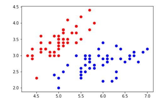
加载好需要的包，使用鸢尾花数据集，为了方便可视化，只取前两个特征，然后将其绘制出来

import numpy as np

import matplotlib.pyplot as plt

from sklearn import datasets

iris = datasets.load_iris()

X = iris.data

y = iris.target

X = X[y<2,:2]

y = y[y<2]

plt.scatter(X[y==0,0],X[y==0,1],color='red')

plt.scatter(X[y==1,0],X[y==1,1],color='blue')

图像如下

首先进行数据的标准化的操作，实例化并fit操作，然后对x进行transform操作，传入x_standard，这样就完成了标准化的操作

from sklearn.preprocessing import StandardScaler

standardScaler = StandardScaler()

standardScaler.fit(X,y)

X_standard = standardScaler.transform(X)

在标准化以后就可以调用SVM算法了，对于线性的SVM，可以直接使用LinearSVC类，然后实例化操作，在进行fit，设置C为10的九次方

from sklearn.svm import LinearSVC

svc = LinearSVC(C=1e9)

svc.fit(X_standard,y)

使用先前的绘制函数并绘制图像

from matplotlib.colors import ListedColormap

def plot_decision_boundary(model, axis):

x0,x1 = np.meshgrid(

np.linspace(axis[0],axis[1],int((axis[1]-axis[0])*100)).reshape(-1,1),

np.linspace(axis[2],axis[3],int((axis[3]-axis[2])*100)).reshape(-1,1)

)

X_new = np.c_[x0.ravel(),x1.ravel()]

y_predict = model.predict(X_new)

zz = y_predict.reshape(x0.shape)

custom_cmap = ListedColormap(['#EF9A9A', '#FFF59D&